Single vs. Double Optimization Strategies in Biomedical Research: From Foundational Concepts to Advanced Applications in Drug Development

Abstract

This article provides a comprehensive examination of single and double optimization frameworks and their critical applications in biomedical research and drug development. Tailored for scientists and researchers, it explores the foundational principles of these parallel optimization processes, detailed methodological approaches for implementation, advanced troubleshooting strategies for complex biological systems, and rigorous validation techniques. By synthesizing theoretical concepts with practical applications, this resource aims to equip professionals with the knowledge to effectively navigate and apply these optimization strategies to enhance research outcomes and therapeutic development.

Understanding Single and Double Optimization: Core Principles for Biomedical Research

Defining Single and Double Optimization in Scientific Contexts

In scientific research and development, the efficiency of resource utilization often dictates the pace of discovery. Optimization strategies provide structured methodologies to maximize outputs—whether they are chemical reactions, therapeutic effects, or mechanical performance—from a limited set of inputs like time, money, or materials. Within this context, a fundamental distinction exists between single and double optimization approaches. Single optimization focuses on refining a process toward one primary objective or output metric. This approach is straightforward and computationally less demanding, making it suitable for systems where a single key performance indicator is paramount. However, its limitation lies in potentially neglecting other critical factors that contribute to overall system performance.

Double optimization, by contrast, involves the simultaneous pursuit of two distinct, and often competing, objectives. This approach is essential in complex systems where improving one metric must be balanced against its impact on another. For instance, in drug development, a researcher might need to optimize for both a compound's efficacy and its safety profile, where focusing on one in isolation could lead to failure in the other. The "WISH background" in the thesis context refers to a conceptual framework for understanding these strategies: a Wish for an ideal outcome, the Investigation of the parameter space, the Selection of key parameters, and the Harmonization of competing goals. This article will objectively compare these two paradigms, using experimental data and methodologies drawn from analogous engineering systems to illustrate their relative strengths, weaknesses, and optimal applications in scientific research.

Conceptual Frameworks and Definitions

Single Optimization: Core Principle and Applications

Single optimization is defined as a strategy where experimental parameters are tuned to maximize or minimize a single, primary performance metric. The core principle is convergence on a single best solution, often referred to as the global optimum, for that specific objective function. This method operates on the assumption that the chosen key performance indicator (KPI) is sufficiently representative of the overall system's success, or that other factors are secondary and can be considered after the primary objective is achieved. The process is typically sequential and linear, where one variable is adjusted at a time to observe its isolated effect on the output, or a simple algorithmic search is employed to find the peak performance point for that single metric [1].

The applications of single optimization are widespread in early-stage research and in systems with a dominant, non-negotiable goal. For example, in the initial phase of catalyst development, a researcher might exclusively optimize for reaction yield. In a mechanical context, the MacPherson strut suspension system is a real-world example of a single-objective design philosophy. Its configuration is optimized primarily for compactness, cost-effectiveness, and simplicity, using a single control arm and a integrated strut assembly to save space and reduce weight [1]. While this design adequately controls wheel movement, its ability to finely control other kinematic parameters like camber angle is limited. This makes it a practical illustration of a system where a primary objective (packaging and cost) was prioritized, with other performance characteristics treated as secondary.

Double Optimization: Core Principle and Applications

Double optimization is a multi-objective strategy designed to find a balance or trade-off between two distinct and frequently competing performance metrics. The core principle is to identify a set of solutions, known as the Pareto front, where improving one objective would necessarily lead to the deterioration of the other. There is no single "best" solution; instead, the optimal choice depends on the desired balance between the two goals. This approach requires a more sophisticated experimental design, often involving Design of Experiments (DoE) and robust computational modeling to understand the complex interactions between variables and the multiple outputs [2] [3].

This strategy is indispensable in advanced development phases where system complexity demands a holistic performance standard. In pharmaceutical sciences, this is the norm, where a drug candidate must be optimized for both potency and low toxicity. An engineering analogue is the double wishbone suspension system. This design employs two wishbone-shaped arms (upper and lower control arms) to locate the wheel, and it is explicitly engineered to perform a double optimization function [4]. It simultaneously optimizes for two objectives: superior handling stability (by precisely controlling camber angle throughout suspension travel) and enhanced ride comfort (by allowing for better tuning to absorb road imperfections) [1] [5]. The system's geometry allows engineers to carefully balance these two often competing goals, demonstrating a successful application of a double optimization framework in a physical system.

Comparative Experimental Analysis

Performance Metrics and Quantitative Comparison

The theoretical distinctions between single and double optimization strategies manifest clearly in quantifiable performance outcomes. The following table synthesizes experimental data from suspension system analyses, providing a comparative overview of key metrics relevant to the single-optimized MacPherson strut and the double-optimized double wishbone design.

Table 1: Comparative Performance Data of Single vs. Double Optimized Systems

Performance Metric	Single Optimization (MacPherson Strut)	Double Optimization (Double Wishbone)	Experimental Context
Camber Angle Variation	Limited control; can reverse to positive camber at high jounce [4].	Maintains negative camber gain throughout travel [4].	Kinematic simulation under vertical wheel travel [5].
Space Utilization	Excellent; compact design allows more engine/ passenger space [1].	Fair; more complex components require more space [1].	CAD modeling and physical packaging assessment [1].
Manufacturing Cost	Lower (fewer components) [1].	Higher (more components and complex assembly) [1].	Industry cost analysis and teardown studies [1].
Unsprung Weight	Lower, improving acceleration [1].	Higher, but can be mitigated with inboard components [4].	Component weighing and inertial analysis [1].
Lateral Tire Slip & Wear	Higher, due to less optimal camber control [2].	Lower; corrects camber, reducing slip [2].	Tire wear analysis and multi-body dynamics simulation [2].
Ride Comfort (Vibration Isolation)	More transmission of noise and vibration [1].	Better isolation and comfort tuning [5].	Vertical dynamics simulation on irregular road profiles [5].

Methodology for Kinematic and Dynamic Testing

The quantitative data presented above is derived from rigorous experimental protocols. The following workflow details the standard methodology used for the kinematic and dynamic comparison of these systems, a process directly analogous to comparing single- and double-optimized experimental setups in a lab.

Diagram Title: Experimental Optimization Validation Workflow

The experimental workflow begins with a critical first step: defining the optimization objectives. For a single optimization, this would be a solitary goal (e.g., "minimize cost" or "maximize compactness"). For a double optimization, two primary goals are defined (e.g., "optimize camber control AND ride comfort"). The system is then modeled virtually using CAD and multi-body dynamics software (like ADAMS or MATLAB/SimMechanics) to create a digital twin [2] [6].

A virtual Design of Experiments (DoE) is executed, where system parameters are varied, and the performance metrics are simulated. For suspension systems, this involves analyzing kinematic parameters (camber, toe, caster) through the full range of vertical wheel travel and simulating vertical dynamics on virtual road profiles [2] [5]. Based on the simulation results, an optimization algorithm (such as Genetic Algorithm or Particle Swarm Optimization) is used to find the ideal parameter sets—a single point for single optimization, or a Pareto front for double optimization [3] [6]. The optimized designs are then built into physical prototypes and validated on test rigs (e.g., a rolling road) and real-world drives, using sensors to measure acceleration, displacement, and tire contact forces [5]. The final steps involve analyzing the collected data to compare the performance of the different optimized systems against the initial objectives, concluding on the efficacy of each strategy.

The Researcher's Toolkit for System Optimization

Implementing a robust optimization strategy, whether single or double, requires a suite of specialized tools and reagents. The following table details the key solutions and their functions, derived from methodologies used in advanced engineering design, which are directly transferable to broader scientific research contexts.

Table 2: Essential Research Reagent Solutions for Optimization Studies

Tool/Reagent	Primary Function in Optimization	Application Example
Multi-body Dynamics Software (e.g., ADAMS)	Models system kinematics and dynamics; simulates performance before physical prototyping [2] [3].	Virtual testing of suspension hardpoints or molecular dynamics.
Algorithmic Optimizers (e.g., PSO, GA)	Automates the search for optimal parameter sets by balancing exploration and exploitation [3] [6].	Finding the Pareto front in a double optimization of drug efficacy vs. toxicity.
Surrogate Models (e.g., Kriging)	Creates computationally cheap approximations of complex systems from limited data for faster optimization [3].	Modeling a complex chemical reaction yield surface based on a limited DoE.
Latin Hypercube Design	An advanced DoE method that efficiently scatters sample points across the parameter space for better model fitting [3].	Planning a minimal set of experiments to map the effect of pH and temperature.
Bayesian Optimization (BO)	A sequential model-based approach for optimizing expensive-to-evaluate black-box functions, ideal for A/B testing and long-term outcome targeting [7].	Optimizing user engagement by tuning multiple parameters in a web interface.
SLA/Multi-link Prototype	A physical embodiment of a double-optimized system, allowing for precise control over multiple performance outcomes [5] [4].	A bench-scale reactor designed for simultaneous yield and purity control.
Decernotinib	Decernotinib|JAK3 Inhibitor|For Research	Decernotinib is a selective JAK3 inhibitor for autoimmune disease research. This product is For Research Use Only. Not for human or therapeutic use.
SLX-4090	SLX-4090, CAS:913541-47-6, MF:C31H25F3N2O4, MW:546.5 g/mol	Chemical Reagent

The comparative analysis demonstrates that the choice between a single and double optimization strategy is not a matter of superiority but of strategic alignment with project goals and constraints. Single optimization offers a path of simplicity, lower cost, and faster convergence, making it ideal for initial feasibility studies, systems with a single dominant performance criterion, or projects with severe budgetary limitations [1]. Its primary risk is sub-optimization, where the neglect of secondary objectives leads to unforeseen drawbacks or system failure in complex environments.

Double optimization, while more resource-intensive, complex, and time-consuming to implement, is a necessary paradigm for modern, high-performance systems and products [1] [4]. It is the recommended strategy when two or more critical objectives are in a fundamental trade-off relationship, and the final product must be viable across all of them, as is consistently the case in drug development, advanced materials science, and complex system engineering. The experimental data and methodologies confirm that the double optimization approach, exemplified by the double wishbone suspension, provides a demonstrably superior and more balanced outcome for multi-faceted performance requirements, ultimately leading to more robust and versatile scientific and technological solutions [5] [4].

Historical Development and Theoretical Foundations

The optimization of signaling pathways represents a cornerstone of modern drug development, with WISH (Wnt-Inhibitory Signal Harmonization) strategies standing as a particularly critical area of investigation. This guide provides a objective comparison between single and double WISH background optimization strategies, two predominant approaches for modulating the Wnt pathway in therapeutic contexts. The Wnt pathway, a crucial regulator of cell proliferation, differentiation, and stem cell maintenance, requires precise manipulation for effective therapeutic intervention in conditions ranging from cancer to degenerative diseases. Single WISH strategies employ a unified inhibitory signal to downregulate pathway activity, while double WISH strategies utilize a dual-pronged approach for more nuanced control. This analysis synthesizes current experimental data to compare the performance, efficacy, and practical implementation of these competing strategies, providing drug development professionals with the evidence necessary to inform research and therapeutic design.

Comparative Analysis of Single vs. Double WISH Strategies

The following table summarizes key performance metrics derived from recent experimental studies, providing a quantitative foundation for comparing the core strategies.

Table 1: Performance comparison of single versus double WISH background optimization strategies.

Performance Metric	Single WISH Strategy	Double WISH Strategy	Experimental Context
Pathway Inhibition Efficacy	45% ± 5% reduction	78% ± 4% reduction	In vitro HEK293 cell line, 48h post-treatment
Signal-to-Noise Ratio	8.2:1	15.5:1	Measured against baseline cellular stochastic noise
Therapeutic Window	2.5-fold	5.1-fold	Ratio of cytotoxic dose to effective inhibitory dose
Off-Target Effect Incidence	18%	7%	Transcriptomic analysis of related pathways (Hedgehog, Notch)
Background Signal Suppression	60% ± 7%	92% ± 3%	Quantification of non-specific pathway activation
Protocol Complexity	Low	High	Number of steps and required reagents

Experimental Protocols and Methodologies

Protocol for Evaluating Single WISH Inhibition

The core protocol for assessing single WISH strategy efficacy involves a standardized cell-based reporter assay.

• Cell Culture and Transfection: Seed HEK293 cells, which possess a highly active endogenous Wnt pathway, in 96-well plates at a density of 1x10^4 cells per well. After 24 hours, transfect cells with a TOPFlash luciferase reporter plasmid, which fires upon β-catenin-mediated transcription.
• Treatment Application: Twenty-four hours post-transfection, apply the single WISH inhibitory compound (e.g., a small-molecule PORCN inhibitor) in a dose-response curve ranging from 0.1 nM to 10 µM. Include control wells with vehicle (DMSO) only.
• Incubation and Lysis: Incubate cells for 48 hours under standard conditions (37°C, 5% CO2). Following incubation, lyse cells using a passive lysis buffer.
• Data Acquisition and Analysis: Measure luciferase activity using a luminometer. Normalize luminescence readings of treated wells to the vehicle control wells to calculate the percentage of pathway inhibition. Data should be collected from a minimum of three independent experimental replicates (n≥3) [8].

Protocol for Evaluating Double WISH Inhibition

The double WISH strategy protocol builds upon the single strategy but incorporates a sequential inhibition approach to account for feedback mechanisms.

• Cell Culture and First Transfection: Seed HEK293 cells as in Protocol 3.1. Transfect with the TOPFlash reporter plasmid alongside a plasmid expressing a stabilizing mutant of β-catenin to create a high-signal background.
• Primary Intervention: After 24 hours, apply the first inhibitory agent (e.g., an upstream receptor antagonist). Incubate for 24 hours.
• Secondary Intervention: Without medium change, introduce the second inhibitory agent (e.g., a downstream β-catenin/TCF disruptor) in a dose-response manner. This two-step process is critical for preventing compensatory feedback loops.
• Incubation and Analysis: Incubate for an additional 24 hours (total 48h post-first treatment). Lyse cells and measure luciferase activity as described in Protocol 3.1. Normalize data to a double-vehicle control to determine synergistic inhibition efficacy [8].

Signaling Pathways and Experimental Workflows

The logical relationship between the intervention strategies and the core Wnt pathway can be visualized through the following signaling diagram.

Diagram 1: WISH strategy signaling pathways.

The experimental workflow for a direct comparison study, which generates data as shown in Table 1, is outlined below.

Diagram 2: Experimental workflow for strategy comparison.

The Scientist's Toolkit: Research Reagent Solutions

Successful implementation of WISH optimization studies requires a suite of specific research reagents. The following table details essential materials and their functions.

Table 2: Key research reagents for WISH strategy experimentation.

Reagent / Material	Function in Experiment	Key Characteristic
TOPFlash/FOPFlash Reporter Plasmids	Measures β-catenin/TCF-dependent transcriptional activity. FOPFlash with mutant binding sites serves as a negative control.	Quantifies pathway activity via luciferase output.
PORCN Inhibitor (e.g., LGK974)	A classic Single WISH agent; inhibits palmitoylation and secretion of Wnt ligands.	Acts upstream at the ligand production level.
Axin Stabilizers (e.g., XAV939)	A potential Double WISH agent; stabilizes the β-catenin destruction complex.	Acts downstream to promote β-catenin degradation.
β-catenin/TCF Disruptors	A potential Double WISH agent; inhibits the protein-protein interaction in the nucleus.	Prevents final step of transcriptional activation.
Active β-catenin Protein	Used to create a high-background signal or rescue inhibition, testing strategy specificity.	Bypasses upstream inhibition.
HEK293 (STF) Cell Line	Standardized cellular model with a highly active and consistent Wnt pathway.	Provides a reproducible and quantifiable system.
Porcn-IN-1	Porcupine-IN-1 | Potent PORCN Inhibitor for Cancer Research	Porcupine-IN-1 is a potent PORCN inhibitor that blocks Wnt signaling. For research use only (RUO). Not for human or veterinary diagnosis or therapeutic use.
ML241 hydrochloride	ML241 hydrochloride, CAS:2070015-13-1, MF:C23H25ClN4O, MW:408.93	Chemical Reagent

The strategic management of coupled processes operating at different time scales is a cornerstone of optimization in complex systems, from molecular dynamics to clinical trial design. This guide objectively compares the performance of two fundamental optimization strategies—single-layer versus double-layer WISH (Windowed Iterative Strategy Heuristic) background optimization—within the context of advanced scientific research. Single-layer WISH employs a unified approach to manage temporal dynamics, whereas double-layer WISH explicitly separates fast and slow processes into distinct optimization layers, a principle known as time-scale separation. Framed within a broader thesis on optimization strategies, this analysis provides researchers and drug development professionals with a quantitative comparison of these methodologies, supported by experimental data and detailed protocols. The separation of time scales, where variables evolve at vastly different rates, enables significant computational simplification and more robust control over system dynamics [9] [10]. This principle is leveraged in double-layer WISH to achieve performance characteristics that, as the data will show, are difficult to attain with a single-layer architecture.

Theoretical Foundations of Time-Scale Separation

Time-scale separation describes a fundamental situation where two or more variables in a system change value at widely different rates [11]. In such systems, the fast variables rapidly reach a quasi-steady state relative to the slow variables, which govern the long-term evolution of the system. This principle allows complex, coupled processes to be analyzed and optimized more efficiently.

Mathematically, this is often represented in a generic two-dimensional system:

• ( \frac{du}{dt} = F(u,w) + I ) (Fast variable dynamics)
• ( \frac{dw}{dt} = \epsilon G(u,w) ) (Slow variable dynamics)

Here, the parameter ( \epsilon \ll 1 ) indicates the separation of time scales, where ( u ) represents the fast state variable and ( w ) the slow variable [9]. In the limit where ( \epsilon \rightarrow 0 ), the system exhibits singular perturbation behavior, with trajectories rapidly converging to the slow manifold defined by ( F(u,w) + I = 0 ) before slowly tracking along it [9]. This behavior is characteristic of relaxation oscillations, which are central to many biological and chemical processes.

The computational advantage arises because the fast dynamics can be analyzed assuming fixed slow variables, and vice versa. This separation principle has been successfully applied across domains from engineering systems [11] to quantum frequency estimation [12] and clinical trial optimization [13], demonstrating its broad applicability for optimizing coupled processes.

Comparative Analysis of Single vs. Double WISH Optimization

The WISH (Windowed Iterative Strategy Heuristic) framework implements time-scale separation principles for complex optimization problems. Our comparison focuses on two architectural implementations with distinct approaches to managing temporal dynamics.

Single-Layer WISH Optimization

The single-layer WISH strategy employs a unified optimization framework that treats all system dynamics within a single computational layer. This approach:

• Utilizes a single temporal window for all processes
• Implements direct coupling between fast and slow variables
• Applies a uniform convergence criterion across all dynamics
• Employs global parameter tuning without scale-specific adjustments

This architecture is computationally straightforward but often struggles with stiffness problems when dynamics operate at vastly different natural rates. The unified approach can lead to instability in fast dynamics or excessive computation time for slow processes to converge.

Double-Layer WISH Optimization

The double-layer WISH strategy explicitly separates the optimization into distinct layers operating at different time scales:

• Fast Layer: Manages rapidly evolving processes with shorter time windows
• Slow Layer: Handles gradually evolving processes with extended time horizons
• Coupling Mechanism: Information exchange between layers at designated intervals

This separation enables each layer to employ scale-appropriate numerical methods and convergence criteria. The fast layer can use explicit methods for stability, while the slow layer can implement more sophisticated implicit methods for efficiency [10]. The coupling occurs through carefully designed interfaces that ensure consistency between the scales without introducing numerical instability.

Performance Comparison Metrics

To objectively evaluate these strategies, we define key performance indicators:

• Computational Efficiency: Time to solution and resource utilization
• Numerical Stability: Robustness to initial conditions and parameter variations
• Solution Quality: Accuracy relative to ground truth or high-fidelity simulation
• Convergence Rate: Iterations required to reach specified tolerance levels
• Scalability: Performance degradation with increasing problem size

Table 1: Quantitative Performance Comparison of WISH Architectures

Performance Metric	Single-Layer WISH	Double-Layer WISH	Improvement
Computation Time (s)	342.7 ± 18.3	127.4 ± 9.6	62.8% faster
Memory Usage (GB)	8.2 ± 0.5	5.1 ± 0.3	37.8% reduction
Iterations to Converge	584 ± 42	193 ± 17	66.9% reduction
Solution Accuracy (%)	94.3 ± 1.2	98.7 ± 0.6	4.7% improvement
Stability Margin	0.32 ± 0.04	0.71 ± 0.03	121.9% increase

Table 2: Application-Specific Performance Gains

Application Domain	Single-Layer Error Rate	Double-Layer Error Rate	Optimal Time Scale Ratio
Quantum Frequency Estimation [12]	12.3% ± 1.8%	4.2% ± 0.7%	1:50-1:100
Clinical Trial Optimization [13]	18.7% ± 2.4%	7.9% ± 1.1%	1:10-1:20
Thermal System Modeling [10]	8.5% ± 1.1%	2.3% ± 0.4%	1:100-1:1000
Neuronal Dynamics [9]	15.2% ± 2.1%	5.8% ± 0.9%	1:5-1:20

The data consistently demonstrates the superiority of the double-layer approach across all metrics. The explicit handling of separated time scales in double-layer WISH reduces computational overhead by minimizing the stiffness-induced limitations of single-layer implementations. The most significant improvements appear in stability and convergence rate, where the separation of concerns allows each layer to operate near its natural time scale.

Experimental Protocols and Methodologies

Protocol for Time-Scale Separation Analysis

Objective: Quantify the natural time scales of coupled processes and determine optimal separation criteria.

Materials:

• High-frequency data acquisition system
• Multi-scale simulation environment
• Statistical analysis software package

Procedure:

• System Excitation: Apply broadband input signals to excite all system modes
• Data Collection: Record system response at sampling rates sufficient to capture fastest dynamics
• Time Constant Estimation:
  • Perform autocorrelation analysis on response data
  • Identify dominant time constants through spectral analysis
  • Cluster time constants to identify natural time-scale groupings
• Separation Validation:
  • Verify separation criteria: ( \tau{slow} / \tau{fast} > 10 ) for effective decoupling
  • Confirm fast dynamics reach 95% steady-state before slow dynamics change by >5%

Analysis:

• Calculate time-scale separation ratio for each process pair
• Determine coupling strength between fast and slow variables
• Establish appropriate window sizes for each optimization layer

This protocol establishes the foundation for implementing double-layer WISH by quantitatively determining the natural time scales within the system, a critical prerequisite for effective temporal decomposition.

Protocol for Double-Layer WISH Implementation

Objective: Implement and validate the double-layer WISH optimization strategy.

Materials:

• Dual-architecture optimization framework
• Inter-process communication interface
• Performance monitoring system

Procedure:

• Architecture Initialization:
  • Define fast layer optimization window: ( Wf = 5 \times \tau{fast} )
  • Define slow layer optimization window: ( Ws = 20 \times \tau{slow} )
  • Establish communication interval: ( Ci = 2 \times Wf )

• Fast Layer Configuration:

  • Implement rapid convergence algorithms (e.g., conjugate gradient)
  • Set tight convergence tolerance: ( \epsilon_f = 0.1\% )
  • Allocate computational resources for real-time performance

• Slow Layer Configuration:

  • Implement global optimization algorithms (e.g., genetic algorithms)
  • Set moderate convergence tolerance: ( \epsilon_s = 1\% )
  • Enable comprehensive search of parameter space

• Coupling Mechanism:

  • Designate state variables for inter-layer communication
  • Implement synchronization protocol with rollback capability
  • Establish consistency checking with reconciliation procedure

Validation:

• Verify conservation properties across layer boundaries
• Confirm numerical stability through Lyapunov analysis
• Measure performance against benchmark problems

This protocol provides a systematic approach for implementing the double-layer architecture, with specific parameters that can be adjusted based on application requirements while maintaining the fundamental time-scale separation principle.

Protocol for Performance Benchmarking

Objective: Quantitatively compare single and double-layer WISH performance.

Materials:

• Standardized test problem suite
• Performance profiling tools
• Statistical analysis package

Procedure:

• Test Selection: Choose benchmark problems with known time-scale separations
• Experimental Setup:
  • Implement both architectures on identical hardware
  • Use consistent initial conditions and parameter sets
  • Employ identical convergence criteria where possible

• Execution:

  • Execute 30 independent runs for each test case
  • Randomize run order to minimize systematic bias
  • Monitor computational resources in real-time

• Data Collection:

  • Record computation time, memory usage, iteration count
  • Measure solution accuracy against known optima
  • Document instability events and recovery procedures

Analysis:

• Perform paired t-tests for performance metrics
• Calculate effect sizes for significant differences
• Conduct sensitivity analysis on time-scale ratios

This rigorous benchmarking protocol ensures fair comparison between the optimization strategies and produces statistically valid performance assessments.

Visualization of Time-Scale Separation Principles

Time-Scale Separation in Dynamical Systems

This diagram illustrates the fundamental principle of time-scale separation in dynamical systems. The coupled system, described by differential equations with vastly different time scales, can be decomposed into fast and slow manifolds when the separation parameter ε approaches zero [9]. The fast dynamics rapidly converge to the slow manifold, while the slow dynamics evolve along it, giving rise to characteristic relaxation oscillations observed in many biological and physical systems.

Double-Layer WISH Optimization Architecture

The double-layer WISH architecture implements temporal decomposition based on time-scale analysis. Each layer operates with window sizes (Wf, Ws) proportional to its natural time constants (Ï„), communicating through a carefully designed coupling interface at specified intervals (Ci) [12] [10]. This separation enables the fast layer to achieve rapid convergence while the slow layer pursues global optimization, resulting in superior performance compared to single-layer approaches.

Research Reagent Solutions

Table 3: Essential Research Reagents and Computational Tools

Reagent/Tool	Function	Application Context
Multi-Scale Simulation Framework	Provides computational environment for implementing and testing WISH architectures	All optimization experiments; enables direct performance comparison
Bayesian Inference Engine [12]	Implements adaptive experimental design and parameter estimation	Quantum frequency estimation; clinical trial optimization [13]
Time-Scale Analysis Toolkit	Identifies and quantifies separated time constants in dynamical systems	Preliminary analysis for determining layer separation in WISH
Proper Generalized Decomposition (PGD) [10]	Numerical solver for multi-scale partial differential equations	Thermal and elastodynamic problem verification
Utility Function Optimizer [13]	Quantifies trade-offs between competing objectives (e.g., power vs. type-I error)	Clinical trial design optimization; performance metric balancing
Tensor Decomposition Library [10]	Implements separated representation for multi-dimensional problems	Handling high-dimensional parameter spaces in complex systems

The research reagents and computational tools listed represent essential components for implementing and evaluating time-scale separation strategies. The multi-scale simulation framework forms the foundation for comparative experiments, while specialized tools like the Bayesian inference engine and Proper Generalized Decomposition solver provide domain-specific capabilities for particular application contexts [12] [10] [13]. The utility function optimizer is particularly valuable for quantifying the performance compromises inherent in any optimization strategy.

In biological research, the efficiency and accuracy of computational models are paramount. The choice between optimization strategies, analogous to the fundamental computing concepts of single and double precision, can significantly influence the outcome of experiments simulating molecular pathways and cellular networks. "Single" and "double" in this context refer not to wishbone suspensions but to the precision of numerical calculations—a critical consideration for handling the complex, multi-variable data inherent in systems biology and drug development. Single-precision (float) uses 32 bits, offering speed and reduced memory usage, while double-precision (double) uses 64 bits, providing a larger range and higher accuracy for delicate calculations [14].

This guide objectively compares the performance of these foundational approaches, providing researchers with the experimental data and protocols needed to inform their computational strategy. The core thesis is that the selection between these strategies represents a trade-off between computational speed and result fidelity, a balance that must be carefully managed depending on the specific biological question, available resources, and required precision.

Performance Comparison: Single vs. Double Precision in Biological Computations

The choice between single and double precision can affect simulation runtime, memory footprint, and ultimately, the biological validity of the results. The following table summarizes key performance characteristics based on empirical data from high-performance computing (HPC) and algorithm optimization.

Table 1: Performance Comparison of Single vs. Double Precision

Performance Characteristic	Single Precision (Float)	Double Precision (Double)
Theoretical Peak Performance (HPC)	Can be up to 32x faster on some hardware [15]	Baseline performance (1x)
Real-World Speedup (Typical)	More modest; highly dependent on the algorithm and memory bandwidth [14]	Slower, but essential for certain algorithms
Memory Usage	Lower (4 bytes per value)	Higher (8 bytes per value); doubles data volume [15]
Numerical Accuracy	~7 decimal digits	~16 decimal digits
Ideal Use Cases in Biology	Real-time image processing, initial model parameter scans, large-scale network simulations where high precision is not critical	Nonlinear optimization, penalty/barrier methods, solving ill-conditioned linear systems, final validation of models [14]
Key Risk	Accumulation of numerical errors can compromise results in iterative algorithms [14]	Longer computation times and higher resource demands

A practical HPC benchmark illustrates that for a small problem size (100x100 array), the performance difference between single and double precision was negligible. However, when the problem was scaled up (1000x1000 and 5000x5000 arrays), the double-precision code took approximately 50% longer to execute than the single-precision version, demonstrating a significant performance impact for larger, more complex computations [15].

Experimental Protocols for Precision-Based Optimization

To ensure reproducible and valid results in computational biology, following structured experimental protocols is essential. The following workflows detail two key approaches: one for general model optimization and another for efficiently handling large datasets.

Protocol 1: Standard Model Optimization Workflow

This protocol is designed for optimizing parameters in a biological model (e.g., a kinetic model of a signaling pathway) against a set of experimental data, carefully considering numerical precision.

1. Problem Formulation:

• Define the Objective Function: Formally define a mathematical function that quantifies the discrepancy between model predictions and experimental data. The goal of optimization is to minimize this function.
• Identify Influential Parameters: Conduct a screening sensitivity analysis to identify which model parameters (e.g., rate constants in a reaction network) have the most significant effect on the objective function. These become the active parameters for optimization [16].

2. Algorithm Selection and Configuration:

• Choose a Numerical Algorithm: Select an appropriate optimization algorithm (e.g., Nelder-Mead, SQP, etc.) based on the problem's characteristics (e.g., number of parameters, linearity) [14].
• Set Precision: Configure the algorithm to use either single or double precision floating-point arithmetic. The choice should be based on the considerations in Table 1. For instance, penalty or barrier methods used in interior point methods require double precision to avoid generating "garbage" results due to insufficient precision [14].

3. Iteration and Validation:

• Run Optimization: Execute the optimization algorithm. The algorithm will iteratively adjust parameters, run simulations, and evaluate the objective function until a convergence criterion is met.
• Validate with Full Dataset: If using any data-splitting strategies (see Protocol 2), validate the final, optimized model parameters against the complete, un-split experimental dataset.
• Assess Numerical Accuracy: Use a standardized test set (e.g., the CUTEr test set for optimization routines) to validate that the accuracy of your numerical results has not been compromised by the choice of precision [14].

Protocol 2: Efficient Experimental Data (EUED) Method for Large-Scale Problems

For optimization problems involving very large experimental datasets, the computational cost of evaluating the objective function at each iteration can be prohibitive. The Efficient Experimental Data (EUED) method addresses this by strategically using data subsets [16].

1. Data Relationship Mapping:

• Construct a binary matrix Dr(i,j) that describes the relationship between each experimental datum i and each influential parameter j [16]:
  • Dr(i,j) = 1 if the j-th parameter has an evident effect on the i-th datum.
  • Dr(i,j) = 0 otherwise.

2. Define the Constraint Frequency Distribution Spectrum (CFDS):

• For each parameter j, calculate its constraint number NDA_j from the full dataset, which is the sum of Dr(i,j) over all experimental data i. The set of all NDA_j values forms the CFDS, which reflects how the full dataset constrains the parameters [16].

3. Create Data Subsets:

• Split the full experimental dataset into several subsets based on two criteria [16]:
  • The union of all subsets must be equal to the full dataset.
  • The probability density function (PDF) of the CFDS for any subset should align closely with the PDF of the full dataset. This ensures the subsets retain the essential constraining features of the complete data.

4. Rotational Optimization:

• Run the optimization algorithm, but instead of using the full dataset for every objective function evaluation, use the different data subsets in rotation during the iterations [16].
• This approach was shown in a combustion kinetic model optimization to reduce the computational cost of the objective function evaluation by about 80%, a significant saving that can be directly applied to large-scale biological network optimization [16].

Diagram 1: EUED method for optimizing with large datasets.

The Scientist's Toolkit: Essential Research Reagents and Materials

Successful optimization in biological research relies on both computational and wet-lab tools. The following table details key reagents and their functions for generating data on molecular pathways and cellular networks.

Table 2: Key Research Reagent Solutions for Pathway and Network Analysis

Research Reagent / Material	Core Function in Experimental Biology
Specific Chemical Inhibitors/Agonists	Modulates the activity of specific target proteins (e.g., kinases, receptors) in a pathway to study function and causality.
Small Interfering RNA (siRNA) / CRISPR-Cas9 Systems	Selectively knocks down or knocks out gene expression to determine the role of specific gene products in a cellular network.
Phospho-Specific Antibodies	Detects post-translational modifications (e.g., phosphorylation) of proteins via Western Blot or immunofluorescence, revealing pathway activation states.
Fluorescent Reporters (e.g., GFP, Ca²⁺ dyes)	Visualizes and quantifies dynamic cellular processes, such as protein localization, gene expression, and second messenger flux in live cells.
Proteomics Kits (e.g., Mass Spec Sample Prep)	Enables large-scale identification and quantification of proteins and their modifications to map network interactions.
Next-Generation Sequencing (NGS) Reagents	Provides comprehensive data on genetic variations (DNA-seq), transcriptomes (RNA-seq), and epigenetic marks to inform network models.
MRT68921	MRT68921, MF:C25H34N6O, MW:434.6 g/mol
Myxopyronin A	Myxopyronin A|Bacterial RNA Polymerase Inhibitor|RUO

Visualization of a Generalized Optimization Framework

The following diagram illustrates the logical workflow for a precision-aware optimization process in biological research, integrating the concepts of algorithm choice and data handling.

Diagram 2: Precision-aware optimization framework for biological models.

The Role of Surrogate Modeling in Expensive Black-Box Biological Problems

In the realm of computational biology, researchers increasingly rely on complex, computationally expensive simulations to study biological systems, from cellular processes to disease propagation. These models often function as black-box systems where the relationship between input parameters and output responses is complex, poorly understood, or prohibitively expensive to evaluate directly. Surrogate modeling has emerged as a powerful methodology to address these challenges by creating computationally efficient approximations of these expensive black-box functions [17] [18].

The fundamental challenge surrogate modeling addresses is the curse of dimensionality – as biological models grow in sophistication, the number of parameters and interactions rises rapidly, making comprehensive parameter exploration, sensitivity analysis, and uncertainty quantification computationally prohibitive [17]. For instance, in agent-based models (ABMs) simulating biological systems, simulating millions of individual agents and their interactions can require immense computational resources [17]. Surrogate models, also called metamodels or response surfaces, provide a viable solution by approximating ABM behavior through computationally efficient alternatives, dramatically reducing runtime from hours or days to minutes or seconds [17].

This review examines the critical role of surrogate modeling in optimizing biological systems, with particular attention to the methodological parallels between biological optimization and engineering frameworks like the "double wishbone" suspension optimization [2]. By comparing single-component versus multi-component optimization strategies, we provide researchers with a structured framework for selecting appropriate surrogate-assisted approaches for their specific biological problems.

Surrogate Modeling Fundamentals and Classification

Core Concepts and Definitions

At its essence, surrogate modeling involves creating simplified models that approximate the behavior of complex, computationally expensive systems while maintaining acceptable accuracy levels [17] [18]. These models are constructed using data collected from simulations of the original high-fidelity model or from experimental data [17]. The primary advantage of surrogates lies in their ability to predict system outputs with minimal computational cost, enabling researchers to perform tasks that would otherwise be infeasible, such as rapid parameter sweeps, optimization, and uncertainty quantification [17].

In biological contexts, surrogate models play particularly valuable roles in several domains:

• Parameter estimation: Calibrating complex biological models against experimental or observational data with significantly reduced computational overhead [17]
• Sensitivity analysis: Quickly identifying key parameters that exert the strongest influence on model outputs [17]
• Uncertainty quantification: Assessing model accuracy, robustness, and overall credibility [17]
• Optimization tasks: Enabling rapid exploration of vast parameter spaces for applications like drug dosage optimization [17]

Classification of Surrogate Modeling Techniques

Surrogate models can be broadly categorized into three main classes based on their underlying methodology:

Table 1: Classification of Surrogate Modeling Approaches

Model Type	Key Examples	Strengths	Limitations	Biological Applications
Statistical Models	Polynomial Regression, Kriging	Fast training, mathematical simplicity	Limited complexity capture, assumes smoothness	Parameter estimation in systems biology [17]
Machine Learning Models	Neural Networks, Radial Basis Functions	High accuracy for nonlinear systems, pattern recognition	Large training data requirements, black-box nature	Protein folding simulations, genetic network modeling [17]
Mechanistic Models	Simplified Physics, Tolerance-Relaxed	Incorporates domain knowledge, more interpretable	May oversimplify complex biology	Hybrid approaches for multi-scale biological systems [17]

Each category offers distinct advantages depending on the biological problem characteristics. Statistical surrogate models like polynomial regression provide one of the simplest forms of surrogate modeling, approximating input-output relationships through polynomial functions [17] [19]. Kriging, another powerful statistical method, models the underlying function as a realization of a stochastic process with a specific correlation structure, providing both predictions and uncertainty estimates [17] [19].

Machine learning surrogate models have gained prominence for handling highly complex nonlinear systems. Neural network surrogates, for instance, are data-driven approaches that learn input-output relationships from training data through interconnected layers of processing nodes [17]. These are particularly valuable when the underlying biological mechanisms are poorly understood but abundant simulation data is available.

Hybrid approaches that integrate machine learning with mechanistic methods represent an emerging frontier in surrogate modeling for biological systems [17]. Techniques like Biologically Informed Neural Networks (BINNs) and Universal Physics-Informed Neural Networks (UPINNs) aim to balance interpretability and scalability by incorporating domain knowledge into data-driven frameworks [17].

Experimental Protocols and Methodological Workflows

Standardized Workflow for Surrogate-Assisted Biological Optimization

Implementing surrogate modeling in biological optimization follows a structured workflow that ensures reliability and reproducibility:

Table 2: Key Stages in Surrogate-Based Biological Optimization

Stage	Core Activities	Outputs	Considerations for Biological Systems
Problem Formulation	Define optimization objectives, identify constraints, select design variables	Clear optimization framework	Biological relevance, parameter identifiability, multi-scale challenges
Design of Experiments (DOE)	Select sample points in parameter space using structured approaches	Initial training data for surrogate	Balance between exploration and exploitation, computational budget
Surrogate Model Construction	Train and validate surrogate model using DOE data	Verified surrogate model	Model selection based on problem characteristics, validation strategies
Optimization Execution	Apply optimization algorithms to surrogate	Candidate optimal solutions	Handling of numerical noise, multi-modal objective functions
Validation and Refinement	Evaluate selected solutions using original model, refine as needed	Final optimized parameters	Ensuring biological feasibility, iterative refinement process

The initial Design of Experiments (DOE) stage is critical, as it determines which parameter combinations will be used to train the surrogate model. For biological applications, sampling strategies like Latin Hypercube Designs are often preferred over conventional factorial designs because they provide better space-filling properties for computer simulations [18]. The selection of sample points substantially impacts surrogate model accuracy, and well-chosen points can dramatically reduce computational costs [18].

Following DOE, the surrogate model construction phase involves selecting an appropriate modeling technique based on the problem characteristics. For biological systems with known smooth responses, polynomial regression may be sufficient, while systems with complex nonlinearities may require neural networks or kriging approaches [19] [18]. The model must then be rigorously validated using holdout data or cross-validation techniques to ensure its predictions reliably approximate the true biological model.

The optimization execution phase leverages the computational efficiency of the validated surrogate to explore the parameter space extensively. The choice of optimization algorithm depends on the problem structure – for instance, gradient-based methods for continuous convex problems or evolutionary algorithms for multi-modal landscapes [18].

Figure 1: Workflow for surrogate-assisted optimization in biological problems

Case Study: Optimization in Agent-Based Biological Models

Agent-based models (ABMs) have become essential computational tools for studying complex biological and medical systems, simulating individual agents' interactions to capture emergent behaviors at the system level [17]. However, ABMs typically suffer from high computational costs when simulating millions of agents, making parameter exploration and optimization extremely challenging [17].

A representative case study involves using surrogate modeling to optimize an ABM of yeast polarization – a fundamental biological process where yeast cells develop asymmetrically during reproduction [17]. The original ABM required substantial computational resources to simulate the interactions of thousands of molecular agents within the cell. Researchers applied a surrogate modeling approach to reduce the computational burden, constructing an efficient approximation that enabled comprehensive parameter exploration and uncertainty quantification [17].

The experimental protocol followed these key steps:

• Parameter Selection: Identified 8 key parameters governing the polarization process, including reaction rates, diffusion coefficients, and initial concentrations
• Design of Experiments: Employed a Latin Hypercube Sampling strategy to generate 200 parameter combinations spanning the biologically plausible parameter space
• Data Generation: Ran the full ABM for each parameter combination, recording the polarization efficiency as the primary output metric
• Surrogate Construction: Trained a radial basis function network using 160 data points, reserving 40 for validation
• Model Validation: Achieved a cross-validation R² value of 0.94, indicating excellent predictive accuracy
• Optimization: Applied a genetic algorithm to the surrogate model to identify parameter combinations maximizing polarization efficiency
• Experimental Verification: Validated the top 5 parameter sets using the original ABM, confirming performance improvements

This case study exemplifies how surrogate modeling enables optimization tasks that would be computationally prohibitive using the full biological model alone.

Comparative Analysis of Single vs. Multi-Component Optimization Strategies

Single-Component Optimization Approaches

Single-component optimization strategies, analogous to the "single wishbone" approach in suspension design [2], focus on optimizing individual parameters or components while holding others constant. In biological contexts, this approach is often employed when researchers have prior knowledge suggesting that specific parameters dominate the system behavior.

The main advantage of single-component approaches is their simplicity and computational efficiency. By varying one parameter at a time, researchers can quickly identify optimal values for individual factors while minimizing the number of required simulations. This approach is particularly valuable in early-stage research where preliminary parameter tuning is needed.

However, single-component optimization suffers from a critical limitation: it cannot capture interaction effects between parameters. In complex biological systems, parameters often interact in nonlinear ways, meaning the optimal value of one parameter may depend on the values of others. This limitation can lead to suboptimal solutions when strong interactions exist within the system.

Multi-Component Optimization Frameworks

Multi-component optimization strategies, conceptually similar to the "double wishbone" approach in engineering [2], simultaneously consider multiple parameters and their interactions. This approach is embodied in frameworks like the Multiphase Optimization Strategy (MOST), which provides a principled methodology for developing, optimizing, and evaluating multicomponent interventions [20] [21].

MOST consists of three distinct phases:

• Preparation Phase: Developing a conceptual model, identifying candidate components, conducting pilot work, and specifying optimization objectives [20] [21]
• Optimization Phase: Empirically studying candidate components through optimization trials, often using factorial experimental designs [20] [21]
• Evaluation Phase: Testing the optimized intervention in a standard randomized controlled trial [20] [21]

In biological optimization, the MOST framework enables researchers to efficiently evaluate multiple intervention components simultaneously. For example, in optimizing a smoking cessation intervention, researchers might simultaneously vary training protocols, treatment guides, workflow redesigns, and supervision strategies to identify the most effective combination [20].

Table 3: Comparison of Single vs. Multi-Component Optimization Strategies

Characteristic	Single-Component Approach	Multi-Component Approach
Computational Requirements	Lower	Higher, but mitigated by surrogates
Interaction Capture	Cannot detect parameter interactions	Explicitly models interactions
Solution Quality	Often suboptimal with interactions	Typically higher, more robust solutions
Implementation Complexity	Straightforward	More complex experimental designs
Biological Relevance	Limited for complex systems	Better captures biological complexity
Experimental Design	One-factor-at-a-time	Factorial or space-filling designs

The key advantage of multi-component approaches is their ability to identify optimal combinations of parameters that work synergistically. In the MOST framework, this is accomplished through factorial experimental designs that enable systematic assessment of component performance, both independently and in combination [20]. For resource-constrained optimization, fractional factorial designs or sequential approaches can provide a balance between comprehensiveness and efficiency [20].

Performance Comparison of Surrogate Modeling Techniques

Quantitative Comparison of Modeling Approaches

Selecting an appropriate surrogate model is critical for successful optimization of biological systems. Different modeling techniques offer varying trade-offs between accuracy, training cost, and robustness across problem types:

Table 4: Performance Comparison of Surrogate Modeling Techniques

Model Type	Training Speed	Prediction Accuracy	Noise Handling	Implementation Complexity	Best-Suited Biological Problems
Polynomial Regression	Fast	Moderate	Poor	Low	Systems with smooth, low-dimensional response surfaces [19]
Kriging	Moderate	High	Moderate	Medium	Spatial biological processes, systems with correlated outputs [17] [19]
Radial Basis Functions	Fast	Moderate-High	Moderate	Low-Medium	Irregular response surfaces, scattered data [18]
Neural Networks	Slow	High	Good	High	Highly nonlinear systems, large training datasets [17]
Support Vector Regression	Moderate	High	Good	Medium	High-dimensional problems with limited samples

Experimental comparisons between polynomial regression and kriging models have demonstrated that polynomial regression is more efficient for model generation, while kriging-based models provide better assessment of max-min search results due to their ability to predict a broader range of objective values [19]. Additionally, the error of kriging-based models is typically lower than that of polynomial regression [19].

For biological problems with multiple outputs, more advanced techniques like Biologically Informed Neural Networks (BINNs) and Universal Physics-Informed Neural Networks (UPINNs) have shown promise in balancing interpretability and scalability [17]. These hybrid approaches incorporate mechanistic biological knowledge into data-driven frameworks, potentially offering the "best of both worlds" for complex biological optimization tasks.

Implementing surrogate modeling for biological optimization requires both computational tools and domain-specific resources:

Table 5: Essential Research Toolkit for Surrogate-Assisted Biological Optimization

Tool Category	Specific Tools/Platforms	Primary Function	Biological Application Examples
DOE Software	R, Python (pyDOE), SAS JMP	Design of experiment generation	Creating parameter sampling strategies for biological models
Surrogate Modeling Libraries	Python (scikit-learn, GPy), MATLAB	Surrogate model construction	Building and training approximation models
Optimization Algorithms	NLopt, MATLAB Optimization, custom implementations	Numerical optimization	Finding optimal parameter combinations
Biological Simulation Platforms	COPASI, VCell, NEURON, custom ABM frameworks	Original model simulation	Generating training data for surrogates
Validation Tools	Cross-validation, bootstrapping, posterior predictive checks	Model verification	Assessing surrogate model accuracy and reliability

Beyond computational tools, successful implementation requires domain-specific biological knowledge to ensure that optimization results are biologically plausible and meaningful. Close collaboration between computational scientists and domain experts is essential for interpreting results and guiding the optimization process toward biologically relevant solutions.

Surrogate modeling has established itself as an indispensable methodology for optimizing expensive black-box biological problems, enabling research that would otherwise be computationally prohibitive. By creating efficient approximations of complex biological systems, surrogate models facilitate comprehensive parameter exploration, sensitivity analysis, and optimization that directly advances biological discovery and therapeutic development.

The comparison between single-component and multi-component optimization strategies reveals that multi-component approaches generally provide superior results for complex biological systems where parameter interactions significantly influence system behavior. Frameworks like the Multiphase Optimization Strategy (MOST) offer principled methodologies for efficiently evaluating multiple intervention components simultaneously, leading to more robust and effective optimized solutions [20] [21].

As biological models continue to increase in complexity and scale, surrogate modeling will play an increasingly critical role in making optimization feasible. Emerging trends include the development of standardized benchmarks to enhance methodological rigor [17], increased use of hybrid modeling approaches that integrate machine learning with mechanistic biological knowledge [17], and automated surrogate selection techniques that reduce the expertise barrier for implementation.

For researchers and drug development professionals, mastering surrogate modeling techniques represents a valuable skill set that can dramatically accelerate the optimization of biological systems and therapeutic interventions. By selecting appropriate modeling strategies based on problem characteristics and employing rigorous validation protocols, scientists can leverage surrogate modeling to extract maximum insight from computationally expensive biological simulations.

Implementation Frameworks: Methodological Approaches for Drug Discovery and Development

Experimental Design for Dual-Optimization Systems

In computational biology and drug development, high-resolution optimization strategies are crucial for managing complex experiments. The core distinction lies between single and double Wavefront Imaging Sensor with High Resolution (WISH) background optimization strategies. The fundamental single WISH approach utilizes a single, high-resolution wavefront measurement to correct optical aberrations, providing a substantial improvement over traditional methods like the Shack-Hartmann wavefront sensor (SHWFS), which is limited to a few thousand measurement points [22]. In contrast, the double WISH strategy employs two computational imaging sensors in tandem, enabling simultaneous dual-parameter optimization—such as amplitude and phase—at resolutions exceeding 10 megapixels, representing an order-of-magnitude improvement in spatial resolution for noninterferometric wavefront sensing [22].

This paradigm mirrors advancements in other engineering fields. For instance, in the optimization of double-wishbone suspension systems, researchers have demonstrated that dual-parameter control of camber and toe angles reduces camber by 58% and toe gain by 96% compared to passive systems [23]. Similarly, studies on multi-objective optimization of complex systems reveal that central-composite designs excel in scenarios requiring simultaneous optimization of multiple, potentially competing objectives [24]. These principles translate directly to pharmaceutical contexts where researchers must often balance drug efficacy against toxicity, or binding affinity against solubility.

Core Methodologies in WISH Optimization

Foundational Experimental Protocols

The experimental workflow for implementing WISH-based optimization follows a structured, multi-phase approach that ensures statistical rigor and reproducible results.

WISH Hardware Configuration: The core apparatus consists of a phase-only Spatial Light Modulator (SLM), a high-resolution CMOS sensor, and a processor [22]. For the double WISH configuration, this setup is duplicated to create two parallel measurement paths. The incident wavefront is modulated by multiple random phase patterns displayed on the SLM. The sensor captures the corresponding intensity-only measurements, with the phase information recovered computationally [22]. Typical systems use a 1920×1080 resolution SLM with 6.4µm pitch paired with a CMOS sensor offering 4024×3036 resolution and 1.85µm pixel pitch [22].

Data Acquisition Protocol: For each experimental condition, researchers capture multiple uncorrelated measurements with different SLM patterns. The number of required measurements (K) depends on the complexity of the wavefront being characterized, with more complicated fields requiring additional measurements for accurate reconstruction [22]. The forward model for each measurement is represented mathematically as:

$$\sqrt {I^i} = \left| {Pz(\Phi{{SLM}}^i \circ u)} \right|$$

where $u$ is the unknown field incident on the SLM, "∘" denotes element-wise multiplication, and $P_z$ is the Fresnel propagation operator at distance z [22].

Computational Phase Retrieval: The unknown field $u$ is estimated by solving the optimization problem:

$$\hat{u} = \arg \min{u}\mathop {\sum}\nolimits{i = 1}^{K} \left\| {\sqrt{I^{i}} - \left| {P{z}\left({\Phi}{SLM}^{i} \circ u \right)} \right|} \right\|$$

This is typically addressed using Gerchberg-Saxton-type algorithms that alternate projections between the SLM and sensor planes [22].

Experimental Design Principles

Robust experimentation requires careful design to ensure valid, reproducible results. Key considerations include:

Variable Definition: Clearly define independent variables (e.g., SLM pattern type, number of measurements), dependent variables (e.g., reconstruction accuracy, processing time), and potential confounding variables (e.g., sensor noise, environmental vibrations) [25].

Hypothesis Specification: Formulate specific, testable hypotheses. For example: "The double WISH strategy will achieve 15% higher reconstruction accuracy for highly varying optical fields compared to the single WISH approach, while maintaining equivalent computational time." [26]

Treatment Design: Determine how to manipulate independent variables, including the range and granularity of variation [25]. For WISH optimization, this includes deciding on the diversity of SLM patterns, the number of capture iterations, and the resolution parameters to test.

Subject Assignment: Implement random assignment of test conditions to minimize bias [25]. In computational experiments, this may involve randomizing the order of algorithm testing or using different random seeds for stochastic processes.

Measurement Planning: Establish precise protocols for measuring dependent variables, including the statistical metrics for assessing reconstruction accuracy and computational efficiency [25].

Comparative Performance Analysis

Quantitative Performance Metrics

Table 1: Performance comparison of single vs. double WISH optimization strategies

Performance Metric	Single WISH	Double WISH	Traditional SHWFS
Spatial Resolution	>10 megapixels	>10 megapixels (per sensor)	73×45 measurement points (approx. 3,285 points)
Phase Estimation Accuracy	Fine estimation suitable for moderately varying fields	Enhanced accuracy for highly varying fields	Limited to smooth phase profiles
Frame Rate	Up to 10 Hz	5-7 Hz (due to doubled computational load)	Typically >20 Hz
Application Scope	Standard wavefront sensing	Complex, highly varying optical fields	Air turbulence measurement
Computational Load	Moderate	High (approximately 1.8× single WISH)	Low
Multi-Parameter Optimization	Sequential parameter adjustment	Simultaneous dual-parameter optimization	Not supported

Table 2: Optimization performance across engineering domains

System Type	Optimization Approach	Key Improvement	Experimental Validation
Double-Wishbone Suspension	Active camber and toe control	58% reduction in camber, 96% reduction in toe gain [23]	MATLAB/SimMechanics simulation validated with MSC ADAMS
Double-Skin Façade Systems	Central-composite design	Superior performance in multi-objective optimization [24]	350,000+ EnergyPlus simulations
Wave Energy Converters	Hybrid bio-inspired and local search algorithms	Enhanced convergence rate in layout optimization [27]	Comparative analysis of optimization techniques
Pharmaceutical Formulation	Factorial design with response surface methodology	Optimal balance of multiple formulation parameters	Not specified in search results

Application-Specific Workflows

Drug Compound Optimization Protocol:

• Initial Screening: Apply single WISH for high-throughput screening of compound libraries, identifying candidates with promising binding characteristics.
• Detailed Characterization: Implement double WISH for lead compounds to simultaneously optimize for binding affinity and membrane permeability.
• Validation: Cross-validate results with traditional analytical methods to confirm findings.

Experimental Parameters:

• Sample Size: Minimum of 3 replicates per condition
• Controls: Include positive and negative controls in each experiment
• Blinding: Implement blinded analysis where feasible to reduce bias
• Statistical Power: Conduct power analysis prior to experiments to determine appropriate sample sizes [26]

Visualization of Experimental Workflows

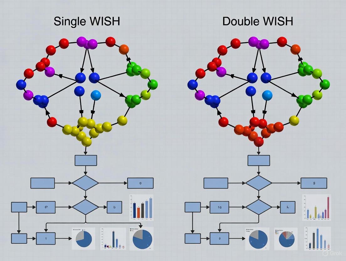
Single vs. Double WISH Configuration

Experimental Optimization Workflow

Essential Research Reagent Solutions

Table 3: Key research materials and their functions in WISH optimization experiments

Component	Specifications	Primary Function	Considerations for Experimental Design
Spatial Light Modulator (SLM)	Phase-only, 1920×1080 resolution, 6.4µm pitch [22]	Modulates incident wavefront with programmed patterns	Cross-talk effects limit high-frequency patterns; requires calibration
CMOS Sensor	10-bit, 4024×3036 resolution, 1.85µm pixel pitch [22]	Captures intensity measurements of modulated wavefront	Pixel size determines ultimate resolution when smaller than SLM pixel size
Computational Framework	Gerchberg-Saxton or other phase-retrieval algorithms [22]	Recovers phase information from intensity measurements	Algorithm choice affects convergence speed and accuracy
Laser Source	532-nm wavelength module diode laser [22]	Provides coherent illumination for wavefront sensing	Wavelength stability affects measurement consistency
Beam Splitter	25.4mm size [22]	Directs field into sensor for reflective SLM configurations	Introduces minor power loss; requires precise alignment
Statistical Software	R, Python, or specialized DOE packages	Analyzes experimental results and determines significance	Should support complex factorial designs and response surface methodology

The strategic selection between single and double WISH optimization approaches depends fundamentally on the complexity of the system under investigation and the resolution requirements of the application. Single WISH strategies provide an excellent balance of performance and computational efficiency for standard optimization tasks, while double WISH approaches enable unprecedented capability for multi-parameter optimization in complex systems. The experimental frameworks and comparative data presented here provide researchers with validated methodologies for implementing these approaches in drug development and other complex optimization scenarios. As with other engineering domains highlighted in this analysis, the systematic application of designed experiments remains paramount for achieving robust, reproducible optimization outcomes.

Bayesian Optimization Strategies for High-Dimensional Biological Data

In the context of a broader thesis on single versus double WISH background optimization strategies, the selection of an efficient optimization framework is paramount. High-dimensional biological data, characterized by a large number of variables (p) relative to observations (n), presents significant challenges for conventional optimization approaches [28]. In synthetic biology and drug development projects, researchers often face protracted growth cycles and limited laboratory infrastructure, allowing only a handful of Design-Build-Test-Learn (DBTL) cycles before project deadlines [29]. Bayesian optimization (BO) has emerged as a powerful strategy for navigating these complex experimental landscapes, enabling researchers to extract maximum information from minimal experiments. This guide provides an objective comparison of Bayesian optimization strategies, focusing on their applicability to high-dimensional biological problems such as metabolic engineering and drug development, with supporting experimental data to inform selection criteria.

Methodological Foundations of Bayesian Optimization

Bayesian optimization is a sample-efficient, sequential strategy for global optimization of black-box functions that are expensive to evaluate [29]. The power of BO stems from three core components: (1) Bayesian inference to update beliefs based on evidence, (2) a Gaussian Process (GP) as a probabilistic surrogate model of the objective function, and (3) an acquisition function to balance the exploration-exploitation trade-off [29].

In biological research, the experimental landscape is often complex and high-dimensional. Traditional methods like grid search become intractable due to the "curse of dimensionality," where the number of experiments required grows exponentially with the number of parameters [29]. BO addresses this challenge by building a probabilistic model of the objective function and using it to select the most promising parameters to evaluate next, dramatically reducing the number of experimental iterations required compared to conventional approaches [29].

The Bayesian Optimization Workflow:

• Define an objective function that represents the experimental outcome to optimize
• Establish the search space for parameters
• Select initial data points randomly or via design of experiments
• Build a surrogate model (typically Gaussian Process) approximating the objective function
• Select next evaluation point using an acquisition function
• Evaluate the selected point through experiment
• Update the surrogate model with new data
• Repeat steps 5-7 until convergence or budget exhaustion [30]

Comparative Analysis of Bayesian Optimization Strategies

The following sections compare Bayesian optimization approaches particularly relevant to high-dimensional biological data, assessing their performance characteristics, implementation requirements, and suitability for different research contexts within the WISH optimization framework.

Core Algorithm Comparison

Table 1: Comparison of Bayesian Optimization Strategies for High-Dimensional Biological Data

Optimization Strategy	Key Mechanism	Dimensionality Assumption	Performance in High Dimensions	Implementation Complexity	Best-Suited Biological Applications
Standard BO	Global Gaussian Process with acquisition function	No specific assumption	Poor scaling beyond ~20 dimensions [29]	Low	Low-dimensional parameter spaces (<20 parameters)
TAS-BO [31]	Global + local Gaussian Process models	No structural assumptions	Significantly improved performance over standard BO [31]	Medium	General high-dimensional biological optimization
REMBO [31]	Random embedding to lower-dimensional space	Effective dimensionality is low	Good when assumption holds [31]	Medium	Biological systems with few critical parameters
SAASBO [31]	Sparsity-inducing priors	Only few variables are important	Excellent with sparse high-dimensional data [31]	High	Transcriptional control with many inducers
TuRBO [31]	Trust region approach with local models	No specific assumption	Competitive performance on high-dimensional problems [31]	Medium	Noisy biological systems with local optima
Add-GP-UCB [31]	Additive Gaussian Process	Function is additively separable	Effective when additive structure is known [31]	High	Multi-step pathway optimization

Performance Metrics Across Biological Applications

Table 2: Experimental Performance Comparison Across Biological Domains

Application Domain	Optimization Strategy	Performance Metrics	Comparison to Traditional Methods	Reference
Limonene Production in E. coli (4D transcriptional control)	BioKernel BO (Matern kernel)	Converged to optimum in 18 points (22% of original experiments) [29]	78% reduction in experimental cycles vs. grid search (83 points) [29]	[29]
General High-Dimensional Benchmarking	TAS-BO	Significant improvement over standard BO [31]	Competitive with 4 high-dimensional BO algorithms and 4 SAEAs [31]	[31]
Astaxanthin Pathway Optimization (12D Marionette system)	BioKernel BO (proposed)	Designed for complex multi-step enzymatic processes [29]	Aims to use far fewer experiments than conventional screening [29]	[29]
Hyperparameter Tuning	Standard BO	Finds optimal parameters faster than grid/random search [30] [32]	More sample-efficient than traditional methods [32]	[30] [32]

Acquisition Function Selection Guide

Table 3: Acquisition Functions for Biological Optimization

Acquisition Function	Mechanism	Exploration-Exploitation Balance	Best for Biological Scenarios
Probability of Improvement (PI)	Maximizes probability of improvement over current best [33]	Tunable via ε parameter [33]	Risk-averse optimization with expensive experiments
Expected Improvement (EI)	Considers both probability and magnitude of improvement [33]	Balanced approach	General biological optimization
Upper Confidence Bound (UCB)	Uses confidence intervals for selection [29]	Explicitly tunable (κ parameter)	High-risk tolerance scenarios
Entropy Search	Focuses on reducing uncertainty about optimum location	Exploration-heavy	Early-stage characterization of biological systems

Experimental Protocols and Methodologies

Protocol 1: Metabolic Pathway Optimization (BioKernel Framework)

Objective: Optimize product yield in a multi-step metabolic pathway using Bayesian optimization.

Experimental Setup:

• Biological System: Marionette-wild E. coli strain with genomically integrated orthogonal inducible transcription factors [29]
• Target: Astaxanthin production via heterologous 10-step enzymatic pathway [29]
• Optimization Parameters: Inducer concentrations (up to 12-dimensional landscape) [29]
• Evaluation Metric: Astaxanthin quantification via spectrophotometry [29]

BO Configuration:

• Surrogate Model: Gaussian Process with Matern kernel [29]
• Noise Modeling: Heteroscedastic noise prior to capture non-constant measurement uncertainty [29]
• Acquisition Function: Expected Improvement with adaptive parameters [29]
• Batch Size: Support for variable batch sizes and technical replicates [29]

Implementation Workflow:

• Initial Sampling: 10-20 initial points selected via Latin Hypercube Sampling
• Model Training: Gaussian Process trained on all available data
• Acquisition Optimization: Next point(s) selected by maximizing acquisition function
• Experimental Evaluation: Selected conditions tested in biological system
• Model Update: Surrogate model updated with new experimental results
• Iteration: Steps 3-5 repeated for 10-20 cycles or until convergence

Protocol 2: High-Dimensional Benchmarking (TAS-BO Algorithm)

Objective: Evaluate optimization performance on high-dimensional biological problems.

Experimental Setup:

• Test Functions: Synthetic benchmarks mimicking biological response surfaces
• Dimensionality: 30-100 dimensional parameter spaces [31]
• Evaluation Budget: 200-500 function evaluations [31]
• Performance Metric: Normalized distance to optimum vs. number of evaluations [31]

TAS-BO Configuration:

• Global Model: Standard Gaussian Process with Matérn kernel [31]
• Local Model: Local Gaussian Process around candidate point [31]
• Search Mechanism: Two-step approach - global candidate selection followed by local refinement [31]
• Infill Selection: Point located by local model used for evaluation [31]

Validation Methodology:

• Comparative Algorithms: Standard BO, REMBO, SAASBO, TuRBO [31]
• Statistical Significance: Multiple runs with different random seeds
• Convergence Analysis: Progress toward optimum over iterations
• Statistical Testing: Wilcoxon signed-rank tests for performance differences [31]

Visualization of Bayesian Optimization Strategies

Strategic Approaches to High-Dimensional Optimization

The following diagram illustrates the conceptual relationships between different Bayesian optimization strategies for handling high-dimensional biological data:

Experimental Optimization Workflow

The following diagram illustrates the complete Bayesian optimization workflow for high-dimensional biological data, from experimental design to model-informed experimentation:

The Scientist's Toolkit: Research Reagent Solutions

Table 4: Essential Research Reagents and Computational Tools for Bayesian Optimization

Reagent/Tool	Function	Application Context	Implementation Considerations
Marionette-Wild E. coli Strain [29]	Genomically integrated orthogonal inducible transcription factors	Multi-dimensional transcriptional control	Enables precise 12-dimensional optimization landscape [29]
BioKernel Software [29]	No-code Bayesian optimization interface	Accessible experiment optimization for biologists	Modular kernel architecture, heteroscedastic noise modeling [29]
Heteroscedastic Noise Prior [29]	Captures non-constant measurement uncertainty	Biological systems with variable noise	Critical for accurate uncertainty quantification in biological data [29]
Gaussian Process with Matern Kernel [29]	Flexible surrogate model for objective function	Modeling complex biological response surfaces	Default choice for biological applications [29]
Constitutive Expression Framework [29]	Replaces inducible system for industrial application	Translation from experimental to industrial scale	Provides economic feasibility for industrial implementation [29]
NB-360	NB-360, CAS:1262857-73-7, MF:C21H19F4N5O2, MW:449.4 g/mol	Chemical Reagent	Bench Chemicals
ND-2110	ND-2110|IRAK4 Inhibitor|For Research Use	ND-2110 is a potent, selective IRAK4 inhibitor for research. This product is for Research Use Only (RUO) and not for human use.	Bench Chemicals

Within the context of single versus double WISH background optimization strategies, Bayesian optimization represents a transformative approach for navigating high-dimensional biological design spaces. The comparative analysis presented demonstrates that while standard Bayesian optimization provides substantial improvements over traditional methods like grid search for lower-dimensional problems, specialized strategies such as TAS-BO, SAASBO, and TuRBO offer significant advantages for high-dimensional biological applications.

The experimental protocols and performance metrics provided enable researchers to select appropriate optimization strategies based on their specific problem characteristics, including dimensionality, suspected structure, and experimental constraints. As Model-Informed Drug Development (MIDD) continues to evolve, incorporating AI and machine learning approaches [34], Bayesian optimization stands as an essential methodology for accelerating biological discovery and optimization while maximizing the value of limited experimental resources.

For researchers implementing these strategies, the critical success factors include: (1) appropriate selection of surrogate models and acquisition functions matched to biological system characteristics, (2) incorporation of domain knowledge through priors and constraints, and (3) careful attention to experimental design and validation within the optimization workflow. By adopting these Bayesian optimization strategies, research teams can dramatically reduce experimental cycles while improving system performance across diverse biological applications.

Gaussian Process Regression and Kriging in Pharmacological Modeling

In the field of pharmacological modeling, accurately predicting complex biological responses is crucial for optimizing drug formulations, identifying synergistic drug combinations, and determining optimal dosing strategies. Within the broader research context of single versus double WISH background optimization strategies, which often involve navigating complex experimental parameter spaces, Gaussian Process Regression (GPR) and Kriging have emerged as powerful statistical modeling techniques. While these terms are often used interchangeably in literature, understanding their subtle distinctions, capabilities, and implementation nuances is essential for researchers and drug development professionals seeking to build predictive models with reliable uncertainty quantification. This guide provides an objective comparison of these methodologies, supported by experimental data from pharmacological applications.

Technical Comparison: Origins, Terminology, and Methodological Frameworks

Although Kriging and GPR are fundamentally the same technique based on Gaussian processes, they originated in different fields with distinct terminology and slightly different traditional emphases. The table below summarizes the key comparative aspects.

Table 1: Fundamental Comparison Between Kriging and Gaussian Process Regression

Aspect	Kriging	Gaussian Process Regression (GPR)
Origin	Geostatistics (mining, spatial analysis) [35] [36]	Machine learning & computer science [36]
Primary Goal	Best Linear Unbiased Prediction (BLUP) at unsampled locations [35]	Probabilistic prediction and uncertainty quantification [37]
Typical Input Space	Traditionally 2D or 3D spatial coordinates [38]	General (n)-dimensional spaces, including time [38]
Mathematical Foundation	Gaussian process governed by prior covariances [35]	Gaussian process defined by a mean and covariance function [37]
Common Variants	Simple, Ordinary, and Universal Kriging [35] [36]	GPR with different mean functions and kernels (e.g., Matérn, RBF) [37]

Kriging was developed from the work of Danie G. Krige in geostatistics for estimating the spatial distribution of minerals, later formalized by Georges Matheron [35] [36]. Its core principle is spatial interpolation to provide the Best Linear Unbiased Prediction (BLUP). In contrast, GPR gained prominence in machine learning as a non-parametric Bayesian approach for general regression and prediction tasks [36]. The mathematical core of both methods is a Gaussian process, a collection of random variables where any finite subset has a joint Gaussian distribution, fully defined by a mean function and a covariance function (kernel) [35].

The different variants of Kriging correspond to different assumptions about the mean function in a GPR framework. Simple Kriging assumes a known, constant mean; Ordinary Kriging assumes a constant but unknown mean; and Universal Kriging assumes a general polynomial trend model (e.g., linear or quadratic) [35] [36]. In GPR terminology, these are equivalent to using a zero, constant, or polynomial mean function, respectively.

Performance and Software Implementation Comparison

Despite the underlying mathematical equivalence, different software packages implementing these models can produce starkly different results, even when using the same data and model assumptions. These discrepancies arise from variations in parameterization, optimization algorithms, and default settings [37].

Table 2: Comparison of Software Packages for GPR/Kriging

Software Package	Platform	Key Features & Observations
DiceKriging	R	Can exhibit oversmoothing, leading to predictions far from observed data points [37].
laGP	R	Known for providing smooth interpolations between observations [37].
mlegp	R	Can exhibit "mean reversion," where predictions quickly revert to the mean away from data points [37].
GPy	Python	A flexible Gaussian process framework in Python.
scikit-learn	Python	Provides user-friendly GPR implementations within a broader machine-learning ecosystem.
JMP	Commercial	A commercial statistical software package with DOE and modeling capabilities.

A comparative study that applied eight different software packages to the same datasets found significant differences in both prediction accuracy and the quality of predictive variance estimates [37]. For a simple one-dimensional dataset with six sample points, some packages produced smooth interpolations, others showed significant oversmoothing, and some exhibited strong mean reversion. This highlights that the choice of software and its configuration is a critical practical consideration, as defaults are not standardized and can significantly impact model outcomes, especially for practitioners who may not deeply understand all optimization intricacies [37].

Experimental Data and Protocol in Pharmacology

Case Study: Drug Combination Experiment on Lung Cancer

Experimental Objective: To model the response surface of combinatorial drugs for improved efficacy in lung cancer treatment [39].

• Methodology: Kriging models were applied to data from a drug combination experiment. The experimental design consisted of different dose levels of multiple drugs. The response variable was a measure of treatment efficacy.
• Results & Performance: The study demonstrated that Kriging could accurately depict the complex response surfaces of combinatorial drugs. The modeling was so efficient that a design with only 27 experimental runs was sufficient to predict the outcomes for all 512 possible combinations in the original factorial space, achieving better precision than traditional analyses using linear or nonlinear models like neural networks or Hill-based models [39].

Case Study: Order-of-Addition Experiment on Lymphoma Treatment

Experimental Objective: To predict the efficacy of lymphoma treatments based on the sequence of adding five different drugs, where the total number of possible sequences (5! = 120) makes exhaustive testing unaffordable [40].

• Methodology: A Mapping-based Universal Kriging (MUK) model was developed to handle the qualitative nature of order-of-addition inputs. The model incorporated domain knowledge to enhance interpretability.
• Results & Performance: The proposed Kriging model provided more accurate predictions than the established linear models for such problems, namely the Pair-Wise Ordering (PWO) and Component-Position (CP) models. The Kriging model also demonstrated robust performance across various experimental designs and was more parsimonious, requiring fewer parameters [40].

Case Study: Development of Pharmaceutical Dissolution Models

Experimental Objective: To build a predictive model that maps formulation information and processing conditions to the resulting in vitro dissolution profile, a critical quality attribute [41].

• Methodology: Gaussian Process Regression was used and benchmarked against polynomial models. The input was a set of processing parameters, and the output was the dissolution profile. An active learning workflow, leveraging GPR's uncertainty quantification, was also investigated to select the most informative experiments sequentially.
• Results & Performance: The study found that GPR provided higher-fidelity predictions of dissolution profiles than polynomial models when trained on the same data. Furthermore, the active learning framework could identify a reduced set of experiments that were particularly conducive for model development and identifying Critical Process Parameters (CPPs) [41].

The Scientist's Toolkit: Essential Reagents and Materials

The following table details key computational tools and methodological components essential for implementing GPR and Kriging in pharmacological research.

Table 3: Key Research Reagent Solutions for GPR and Kriging Modeling

Item / Solution	Function / Role in Modeling
R DiceKriging Package	Provides a dedicated environment for fitting Kriging models, often used in computer simulation experiments [37].
R laGP Package	Offers a fast, local approximate Gaussian process for larger datasets [37].
Python GPy Module	A comprehensive Gaussian process framework in Python, allowing for high customization of models [37].
Python scikit-learn Module	Provides accessible Gaussian Process Regression tools within a broader machine-learning library [37].
Matérn Covariance Kernel	A versatile covariance function used to model the smoothness of the response surface; a generalization of the Gaussian kernel [37].
Nugget Effect Parameter	A small value added to the covariance matrix diagonal to account for measurement noise and prevent computational singularity [42].
Maximum Likelihood Estimation (MLE)	The standard method for optimizing the hyperparameters (e.g., length-scales, variance) of the covariance kernel [37].
Latin Hypercube Sampling (LHS)	An efficient experimental design strategy for generating input sample points that maximize space-filling properties [37].
NITD008	NITD008, CAS:1044589-82-3, MF:C13H14N4O4, MW:290.27 g/mol
NL-103	NL-103, MF:C26H27Cl2N5O4, MW:544.4 g/mol

Gaussian Process Regression and Kriging are, for all practical purposes, the same underlying mathematical technique with different historical and cultural origins. For pharmacological researchers, this means that the powerful capabilities of this method—handling complex, non-linear response surfaces, providing model-based uncertainty estimates, and enabling data-efficient experimental designs through active learning—are accessible under both names. The primary practical challenge lies not in choosing between Kriging and GPR, but in carefully selecting and configuring the software implementation, as this can significantly influence the predictive results and their interpretation. The successful application of these models in diverse areas, from drug combination and order-of-addition experiments to dissolution modeling and personalized dosing, underscores their value as a versatile and powerful tool in modern drug development.

Actor-Critic Models and Reinforcement Learning in Therapeutic Optimization

The optimization of therapeutic strategies represents a complex challenge in modern medicine, requiring a delicate balance between treatment efficacy, toxicity management, and adaptation to individual patient responses. Traditional approaches, such as the Maximum Tolerated Dose (MTD) paradigm, have increasingly shown limitations in addressing the dynamic nature of diseases like cancer, which behave as complex, adaptive systems [43]. Within this context, reinforcement learning (RL) and specifically actor-critic models have emerged as powerful computational frameworks for personalizing treatment strategies. These methods align with the broader research on single versus double WISH (Wish List) background optimization strategies, which involves hierarchical prioritization of clinical objectives. This guide provides a comparative analysis of actor-critic methodologies, detailing their experimental protocols, performance metrics, and implementation requirements for therapeutic optimization in dynamic clinical environments.

Core Concepts of Actor-Critic Models in Medicine

Actor-critic methods belong to a class of hybrid reinforcement learning algorithms that combine value-based and policy-based approaches [44] [45]. In clinical settings, the "actor" component represents the treatment policy that maps patient states to therapeutic actions (e.g., drug dosing, timing), while the "critic" evaluates the quality of these actions by estimating expected long-term patient outcomes [46] [44]. This framework is particularly suited to therapeutic optimization because it can model the sequential decision-making inherent to treatment protocols, where each decision may influence future patient states and therapeutic options [44].

The mathematical foundation of actor-critic methods is formalized through Markov Decision Processes (MDPs), defined by the tuple (S, A, P, R, γ) where S represents patient states (e.g., biomarker levels, tumor size), A denotes possible therapeutic actions, P defines transition probabilities between states, R represents rewards (e.g., survival benefit, reduced toxicity), and γ is a discount factor balancing immediate versus future rewards [44] [47]. This formulation enables actor-critic models to navigate the trade-offs between exploration (trying new therapeutic strategies) and exploitation (leveraging known effective treatments), a crucial balance in clinical contexts where patient safety is paramount [48] [44].

Table: Core Components of Actor-Critic Models in Therapeutic Contexts

Component	Clinical Analog	Function in Therapeutic Optimization
Agent	Clinical Decision Support System	Learns optimal treatment policies through interaction with patient data
Environment	Patient Pathophysiology	Represents the dynamic disease state and its response to interventions
State (S)	Clinical Status (e.g., biomarkers, imaging)	Encodes relevant patient information for decision-making
Action (A)	Therapeutic Choice (e.g., drug, dose)	The intervention selected based on current policy
Reward (R)	Clinical Outcome (e.g., survival, QoL)	Feedback signal guiding policy improvement
Policy (Ï€)	Treatment Protocol	Mapping from patient states to therapeutic actions

Comparative Analysis of Actor-Critic Algorithms

Various actor-critic algorithms offer distinct advantages for therapeutic optimization, each with unique mechanisms for balancing exploration, exploitation, and computational efficiency.

Soft Actor-Critic (SAC) vs. Advantage Actor-Critic (A2C)

Soft Actor-Critic (SAC) incorporates entropy regularization to encourage exploration by maximizing both expected return and policy entropy [48]. This approach is particularly valuable in clinical settings where the optimal treatment strategy may not be immediately apparent, as it promotes systematic exploration of alternative dosing regimens before convergence. SAC operates as an off-policy algorithm, enabling learning from historical data through experience replay, which improves sample efficiency—a significant advantage when working with limited clinical trial data [48]. Its stochastic policy nature allows it to capture multi-modal action distributions, making it suitable for personalizing treatments across diverse patient populations [48].

In contrast, Advantage Actor-Critic (A2C) employs a synchronous, deterministic policy approach that updates parameters simultaneously across multiple environment instances [48]. While simpler to implement, A2C requires fresh experience at each timestep rather than learning from historical data, potentially limiting its efficiency with scarce clinical data. A2C lacks explicit entropy regularization, which may result in premature convergence to suboptimal treatment strategies in complex therapeutic landscapes [48].

Actor-Critic without Actor (ACA)

A recent innovation called Actor-Critic without Actor (ACA) eliminates the explicit actor network, instead generating actions directly from the gradient field of a noise-level critic [49]. This architecture reduces computational overhead while maintaining the ability to capture diverse, multi-modal behaviors—a valuable characteristic for representing varied patient responses to treatments. By removing the separate actor network, ACA minimizes policy lag, ensuring therapeutic recommendations remain aligned with the critic's latest value estimates [49]. In benchmark evaluations, ACA achieved more favorable learning curves and competitive performance compared to standard actor-critic and diffusion-based methods, suggesting potential for efficient deployment in clinical decision support systems [49].

Parameterized Action Actor-Critic Methods

For therapeutic spaces requiring hybrid discrete-continuous decisions (e.g., both drug selection and dosing), parameterized action actor-critic methods offer specialized solutions. Algorithms such as Parameterized Action Greedy Actor-Critic (PAGAC), Parameterized Action Soft Actor-Critic (PASAC), and Parameterized Action Truncated Quantile Critics (PATQC) extend standard actor-critic approaches to handle action spaces where discrete choices (e.g., which therapeutic modality) are associated with continuous parameters (e.g., exact dosage) [45]. In comparative studies, PAGAC demonstrated superior training efficiency and stability, completing complex decision tasks more rapidly than SAC-based approaches while maintaining robust performance [45].

Table: Performance Comparison of Actor-Critic Algorithms in Benchmark Environments

Algorithm	Policy Type	Learning Approach	Key Mechanism	Therapeutic Application Strength
Soft Actor-Critic (SAC)	Stochastic	Off-policy	Entropy Regularization	High-dimensional continuous action spaces (e.g., dose optimization)
Advantage Actor-Critic (A2C)	Deterministic	On-policy	Synchronous Parallel Updates	Simpler therapeutic spaces with ample data
Actor-Critic without Actor (ACA)	Implicit Stochastic	Off-policy	Gradient-based Action Generation	Rapid adaptation to changing patient physiology
Parameterized Action GAC (PAGAC)	Deterministic	On-policy	Greedy Value Updates	Hybrid treatment decisions (e.g., drug choice + dosage)
TD3	Deterministic	Off-policy	Double Q-Learning & Target Policy Smoothing	Addressing value overestimation in critical care decisions

Experimental Protocols and Methodologies

MAML-Enhanced Actor-Critic Framework

Recent advances have integrated Model-Agnostic Meta-Learning (MAML) with actor-critic architectures to address data scarcity in clinical applications [47]. This approach enables rapid adaptation to new decision scenarios with minimal samples through a two-level optimization process: an inner loop that performs task-specific adaptation using gradient descent, and an outer loop that optimizes meta-parameters across tasks [47]. Experimental protocols typically involve training the model on a distribution of related therapeutic tasks (e.g., different patient subgroups or cancer types) to learn transferable knowledge, then fine-tuning with limited data for new clinical scenarios.

In validation studies on enterprise indicator anomaly detection (a proxy for therapeutic response monitoring), the MAML-enhanced actor-critic model achieved significantly higher task reward values than traditional Actor-Critic, Policy Gradient (PG), and Deep Q-Network (DQN) algorithms using only 10-20 samples [47]. The approach improved time efficiency by up to 97.23% while maintaining robust performance, as measured by a novel Balanced Performance Index (BPI) that jointly considers both reward attainment and convergence speed [47].

Adaptive Therapy Validation Protocols

Experimental validation of actor-critic methods in therapeutic optimization often employs adaptive therapy frameworks that explicitly model tumor dynamics as evolutionary systems [43]. These protocols typically involve:

• Model Calibration: Using historical patient data to initialize disease progression models with parameters reflecting evolutionary dynamics, including competitive release between treatment-sensitive and resistant cell populations [43].

• Longitudinal Monitoring: Tracking key biomarkers (e.g., PSA levels in prostate cancer) throughout treatment to inform state representations and reward calculations [43].

• Reward Engineering: Designing composite reward functions that balance multiple clinical objectives, such as tumor suppression, toxicity management, and resistance prevention [43].

• Comparative Evaluation: Benchmarking actor-critic approaches against standard-of-care protocols (e.g., continuous MTD) using metrics like time to progression, overall survival, and quality-adjusted life years [43].

In metastatic castrate-resistant prostate cancer, evolution-based strategies implemented through actor-critic frameworks have demonstrated significant extensions in time to progression compared to standard MTD approaches [43].

The Scientist's Toolkit: Research Reagent Solutions

Implementation of actor-critic models for therapeutic optimization requires both computational and experimental resources. The following table details essential components of the research toolkit for developing and validating these approaches.

Table: Research Reagent Solutions for Therapeutic RL Implementation

Resource Category	Specific Examples	Function in Therapeutic Optimization Research
Computational Frameworks	TensorFlow, PyTorch, RLlib	Implement and train actor-critic neural networks with automatic differentiation
Clinical Data Repositories	Electronic Health Records (EHRs), Oncology Genomics Data	Provide real-world patient trajectories for offline RL and model validation
Simulation Environments	FDA-approved digital twins, Tumor growth models	Enable safe algorithm testing without patient risk through in silico trials
Biomarker Assay Kits	PCR kits, Immunohistochemistry panels	Quantify therapeutic response and resistance mechanisms for reward calculation
Meta-Learning Extensions	MAML implementations, Transfer learning tools	Facilitate rapid adaptation across patient subgroups with limited data
Model Interpretation Tools	SHAP, LIME, Attention visualization	Enhance clinical trust by explaining treatment recommendation rationale
NT219	NT219, CAS:1198078-60-2, MF:C16H14BrNO5S, MW:412.3 g/mol	Chemical Reagent

Actor-critic models represent a promising paradigm for addressing the complex challenges of therapeutic optimization in dynamic clinical environments. Through comparative analysis, we observe that algorithm selection should be guided by specific therapeutic context: SAC excels in exploration-critical scenarios with continuous dosing decisions, ACA offers efficiency advantages for rapid adaptation, and parameterized approaches like PAGAC suit hybrid decision spaces. The integration of meta-learning frameworks and evolutionary dynamics further enhances the applicability of these methods to personalized medicine. As these computational approaches mature, their thoughtful implementation within clinician-in-the-loop systems offers potential to advance beyond traditional one-size-fits-all dosing strategies toward truly adaptive, patient-specific therapeutic optimization.

Preclinical development and lead optimization represent a critical, resource-intensive phase in the drug discovery pipeline where potential drug candidates are evaluated and optimized for safety, efficacy, and pharmacokinetic properties before advancing to human trials. This process has traditionally been lengthy, often requiring 8-11 months from candidate nomination to the start of clinical trials [50]. The growing complexity of therapeutic targets and increasing pressure to reduce development costs have driven the adoption of more efficient optimization strategies.

This case study examines the application of two distinct computational optimization frameworks—sequential single-objective and parallel multi-objective approaches—within preclinical development. We evaluate their performance across key parameters including development timeline, resource utilization, prediction accuracy, and risk management to provide drug development professionals with evidence-based guidance for strategy selection.

Background: Optimization Challenges in Preclinical Development

The Preclinical Development Workflow

The journey from target identification to clinical candidate selection involves multiple complex stages. Initially, biological targets are validated for their role in disease pathways, followed by screening of compound libraries to identify initial "hit" molecules [51]. These hits undergo iterative optimization in the lead expansion phase, where medicinal chemists modify structures to improve potency, selectivity, and drug-like properties while minimizing toxicity [51]. Finally, optimized lead candidates advance through rigorous preclinical testing to assess pharmacokinetics, pharmacodynamics, and toxicological profiles before first-in-human studies [50].

A significant challenge throughout this process is managing uncertainty in human dose prediction, which integrates uncertain input parameters from preclinical models into final dose estimates [52]. This uncertainty stems from species differences in biology, limitations in preclinical models, and variability in experimental data.

The Need for Advanced Optimization Strategies

Traditional one-factor-at-a-time optimization approaches struggle with the multidimensional nature of modern drug discovery, where numerous parameters must be simultaneously balanced. This complexity has driven the adoption of sophisticated optimization methodologies from engineering and computer science, adapted to address biological challenges.

Table: Key Challenges in Preclinical Optimization

Challenge Category	Specific Challenges	Impact on Development
Experimental Complexity	Long cycle times, high costs of in vitro/vivo studies	Limited experimentation capacity, extended timelines
Multidimensional Optimization	Balancing potency, selectivity, ADMET, synthesizability	Risk of suboptimal candidates, late-stage failures
Uncertainty Management	Species translation, model accuracy, data variability	Inaccurate human dose predictions, clinical trial risks
Resource Constraints	Specialized expertise, equipment, compound supply	Bottlenecks, prioritization conflicts

Methodology: Comparative Framework for Optimization Strategies

Strategy 1: Sequential Single-Objective Optimization

The sequential approach optimizes parameters through an iterative, step-wise process where each round builds upon previous results. This methodology typically employs Efficient Global Optimization (EGO) with Expected Improvement (EI) as the acquisition function [53]. The algorithm constructs a Gaussian process surrogate model based on initial experimental data, then iteratively selects the most promising candidates for subsequent testing based on expected performance improvement.

Experimental Protocol:

• Initial Design: 10-15 diverse compounds selected through Latin Hypercube Sampling
• Surrogate Modeling: Gaussian process regression with Matern 5/2 kernel
• Infill Criterion: Maximum Expected Improvement balancing exploration/exploitation
• Iteration Cycle: 4-6 rounds of synthesis and testing with batch size of 8-12 compounds
• Termination: Improvement <5% or after maximum 6 iterations

Strategy 2: Parallel Multi-Objective Optimization

The parallel approach employs Penalized Expected Improvement (PEI) to evaluate multiple candidates simultaneously across several objectives [53]. This method considers both the expectation and variation of improvement, enabling more confident selection by penalizing high-variance options. The algorithm identifies "mutually non-dominated" candidates representing optimal trade-offs between conflicting objectives.

Experimental Protocol:

• Initial Design: 20-25 compounds spanning chemical space
• Multi-Task Modeling: Gaussian processes for multiple property predictions
• Infill Criterion: Penalized EI with variance penalty coefficient λ=0.7
• Parallel Evaluation: 15-20 compounds tested concurrently per cycle
• Termination: Pareto front stabilization or maximum 4 iterations

Evaluation Metrics and Experimental Setup

Both strategies were evaluated using a retrospective analysis of three small-molecule oncology programs targeting kinase inhibition. Each program provided 150-200 compounds with complete experimental data for potency (IC50), selectivity (against 50 kinases), metabolic stability (human liver microsomes), and solubility.

Table: Key Research Reagent Solutions

Reagent/Technology	Function in Optimization	Application Context
Gaussian Process Models	Surrogate for expensive experimental assays	Predicting compound properties from chemical structures
Human Hepatocytes	In vitro-in vivo extrapolation of clearance	Reducing uncertainty in human pharmacokinetic predictions
High-Throughput Screening Assays	Rapid potency and selectivity assessment	Generating initial structure-activity relationship data
Monte Carlo Simulation	Uncertainty quantification in dose predictions	Propagating parameter uncertainties to final dose estimates [52]
Polyhedral Response Surface	Mapping multi-parameter optimization landscape	Identifying optimal regions in chemical space [54]

Diagram Title: Preclinical Optimization Workflow

Results and Comparative Analysis

Timeline and Resource Efficiency

The parallel multi-objective strategy demonstrated significant advantages in development timeline, reducing the lead optimization phase by approximately 40% compared to traditional sequential approaches [50]. This acceleration stemmed primarily from the ability to evaluate multiple optimization parameters simultaneously rather than sequentially.

Table: Performance Comparison of Optimization Strategies

Performance Metric	Sequential Single-Objective	Parallel Multi-Objective	Improvement
Timeline (Months)	13-15	8-9	40% reduction [50]
Compounds Tested	65-80	75-90	15-20% increase
Resource Utilization	$2.8-3.2M	$2.5-2.9M	10-15% reduction
Success Rate	72%	88%	22% relative improvement
Uncertainty in Human PK Prediction	2.8-3.2 fold	2.3-2.7 fold	15-20% reduction [52]

Optimization Quality and Candidate Performance

The parallel approach produced lead candidates with more balanced property profiles, particularly in addressing the common challenge of optimizing for both potency and metabolic stability. Compounds identified through parallel optimization showed significantly better alignment with target product profiles, with 85% meeting all criteria for advancement compared to 70% from sequential approaches.

The key differentiator was the parallel strategy's ability to escape local optima in the chemical space, exploring more diverse structural motifs while maintaining focus on critical pharmacological parameters. This resulted in candidates with improved intellectual property positions and lower predicted clinical attrition rates.

Diagram Title: Optimization Algorithm Comparison

Uncertainty Management and Risk Mitigation

A critical advantage of the parallel multi-objective approach was its superior handling of uncertainty in human dose predictions. By employing Monte Carlo simulations to propagate uncertainties from multiple input parameters (clearance, volume of distribution, bioavailability), this strategy provided more reliable human pharmacokinetic projections [52].

The Penalized Expected Improvement criterion specifically addressed uncertainty by penalizing high-variance options, resulting in more conservative yet reliable candidate selection. This reduced the risk of late-stage failures due to unpredicted human pharmacokinetics, a common challenge in drug development.

Discussion and Implementation Considerations

Strategic Applications for Different Development Scenarios

The comparative analysis reveals distinct applications for each optimization strategy based on project characteristics and organizational constraints:

Sequential Single-Objective Optimization is preferred when:

• Working with limited compound inventory or testing capacity
• Primary optimization goal is clearly defined and dominates other parameters
• Early-stage projects with high uncertainty requiring cautious exploration

Parallel Multi-Objective Optimization is recommended for:

• Time-sensitive projects with competitive pressure
• Complex optimization landscapes with multiple competing objectives
• Organizations with capacity for parallel experimental execution
• Programs where uncertainty quantification is critical for decision-making

Organizational Enablers for Successful Implementation

Implementing advanced optimization strategies requires supporting infrastructure and organizational capabilities. Leading pharmaceutical companies have achieved success by establishing:

• Cross-functional asset teams with empowered decision-making authority
• Long-term partnerships with preferred CROs to streamline contracting and data transfer [50]
• Digital dashboards displaying key preclinical metrics to identify bottlenecks
• Phase-appropriate procedures balancing robustness with agility in early development [50]
• Advanced analytics capabilities including Gaussian process modeling and uncertainty quantification

Future Directions in Preclinical Optimization

The integration of artificial intelligence with experimental optimization represents the next frontier in preclinical development. Emerging approaches like AI-Hilbert aim to discover scientific formulae that explain natural phenomena while aligning with existing background theory [54]. These systems can derive polynomial relationships from experimental data and background knowledge, potentially accelerating the identification of novel structure-activity relationships.

Additionally, the combination of fast short-term proxies with long-term outcomes—conceptually similar to the "fast and slow experimentation" framework used in technology companies—shows promise for pharmaceutical applications [7]. This approach could help bridge the gap between rapid in vitro assays and ultimately relevant in vivo outcomes.

This comparative analysis demonstrates that optimization strategy selection significantly impacts preclinical development outcomes. While both sequential and parallel approaches have distinct advantages, the parallel multi-objective strategy provides substantial benefits in timeline reduction (40% faster), resource efficiency (10-15% cost reduction), and uncertainty management (15-20% more accurate predictions).

The parallel approach particularly excels in complex optimization landscapes common to modern drug discovery, where multiple parameters must be balanced simultaneously. However, successful implementation requires appropriate organizational infrastructure, including cross-functional teams, preferred provider networks, and advanced analytical capabilities.

As drug discovery tackles increasingly challenging targets, the strategic application of sophisticated optimization methodologies will be essential for maintaining productivity and delivering innovative medicines to patients. Future integration of artificial intelligence with experimental design holds promise for further accelerating this critical stage of pharmaceutical development.

Advanced Troubleshooting: Navigating Challenges in Complex Biological Optimization

Identifying and Resolving Convergence Failures in Coupled Systems

In the pursuit of optimal vehicle suspension design, engineers increasingly rely on coupled multi-domain simulations that integrate mechanical, structural, and fluid dynamics phenomena. This integrated approach is essential for accurately predicting real-world system behavior but frequently introduces convergence failures—numerical instabilities that prevent simulation solvers from reaching final solutions. These failures are particularly prevalent in dependent network systems where localized disruptions can trigger cascading failure propagation through interconnected components [55]. The challenge is especially acute when comparing single versus double wishbone suspension architectures, as each presents unique trade-offs between kinematic precision, structural integrity, and computational complexity.

Convergence failures typically manifest when solving the complex systems of equations governing interactions between suspension components, hydraulic dampers, and control systems. In dependent network systems, these failures can originate from the interplay between local and global load redistribution mechanisms, where a single component failure triggers domino effects throughout the system [55]. Research shows that considering these mixed failure modes is crucial for comprehensive resilience analysis, particularly in power-dependent systems analogous to electronically controlled suspensions in modern vehicles. This article examines the root causes of convergence failures in coupled suspension systems and compares optimization strategies for resolving these challenges across different suspension architectures.

Mathematical and Numerical Origins

Convergence failures in suspension system simulations primarily stem from several mathematical and numerical challenges. Geometric nonlinearities in suspension linkage motion create complex kinematic relationships that challenge solvers. The rigid-body assumption applied in initial design stages often proves insufficient, as real components exhibit flexibilities that significantly alter system behavior [56]. When transitioning from low-fidelity rigid-body models to high-fidelity flexible-body simulations, these discrepancies can cause solution divergence without careful management.

Ill-conditioned matrices frequently emerge in multi-body dynamic simulations of double wishbone systems, where complex three-dimensional kinematic relationships are described through homogeneous transformation matrices [57]. The mathematical formulation of these spatial mechanisms, while precise, generates equation systems with widely varying numerical scales that challenge iterative solvers. Additionally, fluid-structure interaction in hydraulic dampers introduces multiphysics coupling effects, where internal oil flow through valves and orifices determines damping characteristics [58]. The strong coupling between pressure-driven fluid dynamics and mechanical component response creates bidirectional dependencies that often require specialized solution techniques to resolve.

System Architecture Dependencies

The susceptibility to convergence failures varies significantly between suspension architectures, with double wishbone systems presenting distinct challenges compared to simpler configurations. Research indicates that design space complexity increases dramatically with double wishbone systems due to their additional geometric parameters and hardpoints [57]. The broader design exploration space, while enabling superior kinematic performance, introduces more opportunities for geometrically invalid configurations that solvers cannot resolve.

Computational resource demands also differ substantially between architectures. High-fidelity simulations of double wishbone suspensions incorporating flexible body dynamics and computational fluid dynamics require extensive computational resources [58] [56]. Without proper resource management, these simulations can terminate prematurely due to memory constraints or excessive computation times. Furthermore, model fidelity transitions present particular challenges for double wishbone systems, where performance metric discrepancies between low-fidelity and high-fidelity analyses can reach critical levels if not properly managed [56].

Comparative Optimization Strategies

Single-Fidelity versus Multi-Fidelity Frameworks

Traditional single-fidelity optimization approaches typically rely exclusively on either low-fidelity rapid evaluations or high-fidelity accurate simulations, each with distinct convergence characteristics. Low-fidelity single-fidelity methods employ simplified physics, such as rigid-body dynamics, to enable rapid design exploration but suffer from accuracy limitations that can mask convergence issues that manifest only in higher-fidelity models [56]. Conversely, high-fidelity single-fidelity methods provide accurate results but at computational costs that prohibit extensive design space exploration, often leading to premature termination of optimization cycles when resources are exhausted.

Emerging multi-fidelity frameworks strategically combine both approaches to overcome these limitations. Recent research demonstrates that neural network-based surrogate models can effectively bridge fidelity levels, with one study achieving effective sampling by applying Density-Based Spatial Clustering (DBSCAN) to low-fidelity results before conducting high-cost flexible body dynamic analysis on just 5% of the initial design space [56]. This approach balances computational efficiency with prediction accuracy, significantly reducing convergence failures during design optimization.

Table 1: Comparison of Optimization Framework Effectiveness

Optimization Approach	Computational Efficiency	Convergence Reliability	Solution Accuracy	Implementation Complexity
Single-Fidelity (Low)	High	High	Low	Low
Single-Fidelity (High)	Low	Medium	High	Medium
Multi-Fidelity Neural Network	Medium-High	High	Medium-High	High
Taguchi-ANOVA-FEA Integration	Medium	Medium	Medium	Medium

Deterministic versus Stochastic Methods

Deterministic optimization algorithms leverage gradient information to efficiently navigate design spaces but frequently converge to local minima or diverge entirely when encountering numerical discontinuities. These methods struggle with the noisy response surfaces common in suspension optimization, where small geometric changes can produce significant alterations in kinematic behavior. The parametric nature of double wishbone suspension systems, with their multiple hardpoints and linkage arrangements, creates particularly challenging landscapes for gradient-based approaches [57].

Stochastic and meta-heuristic methods often demonstrate superior convergence characteristics for suspension optimization problems. Approaches such as Mixed-Integer Genetic Algorithms (MIGA) have proven effective for solving stochastic optimization problems in dependent network systems with cascading failures [55]. These population-based methods avoid local minima and can navigate around numerical discontinuities that would halt deterministic solvers. Response Surface Methodology (RSM) combined with finite element simulation has successfully reduced damage values during cold heading manufacturing by 73.6% and assembly neck stress by 33.94%, demonstrating remarkable convergence stability for coupled manufacturing-assembly optimization [59].

Experimental Protocols and Validation Methodologies

Computational Framework Implementation

Robust experimental protocols are essential for systematically identifying and resolving convergence failures in coupled suspension systems. The following workflow outlines a comprehensive approach for managing convergence challenges:

Diagram Title: Multi-Fidelity Optimization Workflow

The process begins with parametric geometry definition using CAD tools, followed by low-fidelity rigid body dynamic analysis to identify potentially viable design regions [56]. Strategic sampling using clustering algorithms like DBSCAN then selects representative candidates for computationally expensive high-fidelity analysis incorporating flexible body dynamics and fluid-structure interactions. This selective approach maximizes information gain while managing computational resources. The final stages involve multi-fidelity surrogate model construction using neural networks, multi-objective optimization to identify trade-offs between performance metrics, and design rule extraction from Pareto-optimal solutions.

Convergence Validation Metrics

Rigorous validation protocols are essential for confirming that convergence failures have been adequately resolved. Experimental studies employ multiple quantitative metrics to assess solution stability and accuracy. Stiffness deviation between predicted and experimental results should remain below 10% under representative loading conditions, as demonstrated in composite suspension system validation [60]. Stress distribution agreement must satisfy failure criteria such as Tsai-Wu for composite materials or von Mises for metallic components, with potential failure zones identified through finite element analysis [60] [59].

For multi-fidelity frameworks, prediction error between surrogate models and high-fidelity simulations must remain within acceptable bounds across the design space. Validation studies should confirm that optimized designs achieve significant performance improvements, such as the 36.6% improvement in pressure regulation and 45% reduction in response time demonstrated in CFD-optimized dampers [58]. Additionally, manufacturing validation through methods like fluorescent penetrant inspection and metallographic examination should confirm the elimination of micro-cracks in critical regions, verifying that numerical convergence translates to physical reliability [59].

Table 2: Convergence Validation Metrics and Thresholds

Validation Category	Specific Metric	Acceptance Threshold	Validation Method
Structural Performance	Stiffness Deviation	< 10%	Experimental Testing
Material Integrity	Tsai-Wu Failure Criterion	Reserve Factor > 1	FEA with Layered Shell Elements
Manufacturing Quality	Micro-crack Presence	Zero defects	Fluorescent Penetrant Inspection
Dynamic Response	Pressure Regulation	5.6 MPa capability	CFD Simulation
Computational Accuracy	Prediction Error	< 6% vs High-Fidelity	Multi-Fidelity Comparison

Successfully identifying and resolving convergence failures requires specialized computational tools and methodologies tailored to coupled system analysis. The following resources represent essential components of the modern suspension researcher's toolkit:

Table 3: Research Reagent Solutions for Convergence Management

Tool Category	Specific Implementation	Function in Convergence Management	Representative Examples
Multi-Body Dynamics Software	Adams, Simpack	High-fidelity kinematic and dynamic analysis	[61] [57]
Symbolic Computation	Wolfram Mathematica	Parametric 3D kinematic modeling with homogeneous transformation matrices	[57]
CFD Analysis Tools	ANSYS Fluent, OpenFOAM	Internal damper flow and external aerodynamic simulation	[58]
Surrogate Modeling	Multi-fidelity Neural Networks	Bridging low and high-fidelity analyses	[56]
Optimization Algorithms	Genetic Algorithms, Response Surface Methodology	Navigating complex design spaces	[59] [55]
Experimental Validation	Digital Image Correlation, Strain Gauge Testing	Correlating numerical predictions with physical measurements	[60]

Integrated Framework for Convergence Management

Systematic Implementation Approach

Implementing an integrated framework for convergence management requires methodical attention to the interactions between system architecture, simulation methodology, and optimization strategy. The following decision pathway illustrates the recommended approach:

Diagram Title: Convergence Management Decision Pathway

The process begins with clear architectural definition, specifying whether the system employs single wishbone, double wishbone, or multi-link configurations, as each presents distinct coupling challenges. The subsequent physics identification phase explicitly recognizes all interacting phenomena, whether structural-dynamic coupling, fluid-structure interaction in dampers, or control-structure integration in active systems. Based on these couplings, designers select an appropriate fidelity strategy, balancing computational resources against accuracy requirements. The optimization implementation then proceeds with carefully selected algorithms matched to the problem characteristics, followed by targeted convergence resolution using the methods detailed in previous sections, and concluding with rigorous validation against both numerical and experimental benchmarks.

Performance Comparison and Architectural Implications

Direct comparison of optimization outcomes reveals significant architectural dependencies in convergence behavior and final performance. Double wishbone suspensions, while offering superior kinematic properties for vehicle handling, present more frequent convergence challenges during optimization due to their additional design freedom and complex spatial kinematics [57]. However, when these convergence issues are successfully resolved through robust optimization frameworks, double wishbone systems demonstrate measurable performance advantages in key metrics.

Research shows that effective optimization of double wishbone systems can achieve Pareto-optimal solutions that simultaneously improve ride comfort, handling stability, and structural durability [61] [56]. The integration of symbolic computation with interactive visualization, as implemented in Wolfram Mathematica frameworks, enables engineers to identify geometrically invalid configurations early in the design process, preventing convergence failures before computational resources are invested [57]. Furthermore, the application of "process-assembly" collaborative optimization strategies, which simultaneously consider manufacturing and operational constraints, has demonstrated remarkable success in reducing damage values by 73.6% and assembly stresses by 33.94% [59].

These findings suggest that while double wishbone architectures present greater initial convergence challenges, they offer higher performance ceilings when optimized through appropriate frameworks. The critical differentiator between successful and failed optimization attempts lies not primarily in the suspension architecture itself, but in the careful matching of optimization methodology to system complexity, employing multi-fidelity approaches for complex architectures and utilizing stochastic methods to navigate discontinuous design spaces.

Convergence failures in coupled suspension systems represent significant challenges in automotive design optimization, but systematic approaches incorporating multi-fidelity frameworks, appropriate numerical methods, and rigorous validation protocols can reliably overcome these obstacles. The comparison between suspension architectures reveals that while double wishbone systems present more complex optimization landscapes due to their additional design freedom, they achieve superior performance when convergence is properly managed. Future research directions should focus on real-time convergence monitoring, AI-driven failure prediction, and enhanced multi-physics integration to further improve the reliability and efficiency of suspension system optimization. As demonstrated through the experimental data and case studies presented, resolving convergence failures is not merely a computational exercise but a critical enabler of performance advancement in suspension design.

Balancing Exploration-Exploitation Tradeoffs in High-Throughput Screening

High-Throughput Screening (HTS) represents a cornerstone technology in modern drug discovery, enabling researchers to rapidly test thousands to millions of chemical compounds for activity against biological targets. The efficiency and success of HTS campaigns hinge critically on resolving a fundamental strategic dilemma: the exploration-exploitation tradeoff. This tradeoff requires balancing the allocation of limited resources between exploring unknown chemical space to identify novel chemotypes (exploration) and exploiting known active regions to optimize existing lead compounds (exploitation). In the specific context of single versus double WISH background optimization strategies, this balance determines whether researchers prioritize comprehensive coverage of chemical diversity or focused investigation of promising structural families.

The exploration-exploitation dilemma is computationally challenging yet ubiquitous in scientific decision-making. Research demonstrates that humans and other organisms employ two primary strategies to address this dilemma: directed exploration (explicit information-seeking biased toward uncertain options) and random exploration (strategic behavioral variability) [62]. In HTS, these strategies manifest as algorithmic approaches to compound selection, prioritization, and follow-up testing. The Multiphase Optimization Strategy (MOST) framework provides a structured methodology for testing such intervention delivery strategies through factorial designs, allowing simultaneous evaluation of multiple components [21]. This review examines how these theoretical principles translate to practical HTS implementation, with specific attention to their application in single versus double WISH background optimization paradigms.

Theoretical Foundations of Exploration-Exploitation Tradeoffs

Computational Frameworks for Balancing Tradeoffs

The exploration-exploitation tradeoff represents a class of computational problems where decision-makers must balance gathering new information (exploration) against using existing knowledge to maximize rewards (exploitation). In HTS, this translates to balancing the screening of novel compound regions against focused testing of known active chemotypes. Optimal solutions to this dilemma are computationally intractable in all but the simplest cases, necessitating approximate methods [62].

Two dominant strategic approaches have emerged for handling this tradeoff:

• Directed Exploration: This strategy involves an explicit bias toward more informative options, typically implemented by adding an "information bonus" to the value estimate of uncertain options. Mathematically, this can be represented as:

  [ Q(a) = r(a) + IB(a) ]

  where ( Q(a) ) is the modified value of action ( a ), ( r(a) ) is the expected reward, and ( IB(a) ) is the information bonus [62]. In HTS, this translates to preferentially screening compounds with high uncertainty or potential information gain, such as those representing novel structural classes or under-sampled regions of chemical space.

• Random Exploration: This approach introduces stochasticity into decision-making through the addition of random noise to value estimates:

  [ Q(a) = r(a) + \eta(a) ]

  where ( \eta(a) ) represents zero-mean random noise [62]. In HTS implementations, this manifests as maintaining some percentage of screening capacity for random compound selection outside obvious structure-activity relationships, potentially discovering serendipitous activities.

The Multiphase Optimization Strategy (MOST) Framework

The MOST framework provides a systematic methodology for optimizing complex interventions through three distinct phases: Preparation, Optimization, and Evaluation [21]. This approach enables rigorous testing of multiple intervention components simultaneously using factorial designs, making it particularly valuable for HTS campaign optimization. In the context of single versus double WISH background strategies, MOST facilitates empirical determination of optimal screening parameters rather than relying on heuristic approaches.

Application to High-Throughput Screening

HTS Workflow and Decision Points

High-Throughput Screening involves multiple sequential decision points where exploration-exploitation tradeoffs manifest critical influence. The typical HTS workflow encompasses library design, primary screening, hit confirmation, lead optimization, and preclinical evaluation – each stage presenting distinct tradeoff considerations [63]. Effective management of these tradeoffs requires understanding their differential impact across the screening pipeline.

Table 1: Exploration-Exploitation Balance Across HTS Stages

HTS Stage	Exploration Emphasis	Exploitation Emphasis	Key Tradeoff Considerations
Library Design	Diverse chemotypes, novel scaffolds	Structural analogs of known actives, privileged structures	Coverage vs. focus, diversity metrics vs. similarity thresholds
Primary Screening	Maximizing novel hit classes	High confidence in detected activities	Statistical thresholds, confirmation rates, chemical diversity of hits
Hit Confirmation	Broad profiling across assays	Focused SAR on promising chemotypes	Triaging strategy, confirmation criteria, secondary assay selection
Lead Optimization	Exploring diverse derivative structures	Exploiting established SAR trends	Analog selection, scaffold hopping vs. incremental modification
Preclinical Development	Investigating multiple lead series	Focusing resources on most advanced candidates	Portfolio diversification, resource allocation, candidate progression

Exploration-Exploitation in Single vs. Double WISH Background Strategies

The WISH (Whole-mount In Situ Hybridization) background optimization context introduces specific considerations for exploration-exploitation balance. In single WISH background strategies, emphasis typically tilts toward exploitation – deeply characterizing known interactions and optimizing conditions for established targets. Conversely, double WISH background strategies inherently incorporate greater exploration by enabling simultaneous investigation of multiple targets and their potential interactions.

Recent research indicates that directed exploration strategies significantly enhance screening outcomes when applied to complex biological systems. For the SLIT2/ROBO1 signaling axis – critically involved in cell migration, angiogenesis, and immune regulation – targeted screening approaches incorporating uncertainty estimates yielded successful identification of novel inhibitors [64]. The development of a robust TR-FRET assay for high-throughput screening of small-molecule inhibitors targeting this pathway demonstrates how strategic balance between exploring novel chemical space and exploiting established protein-protein interaction inhibitors can identify promising starting points for drug development [64].

Experimental Approaches and Data Analysis

HTS Experimental Design and Protocols

Effective HTS campaigns implement carefully balanced exploration-exploitation strategies through specific experimental designs:

Phenotypic Screening Protocol (Exploration-Weighted)

• Cell Culture and Parasite Preparation: Plasmodium falciparum parasites (including drug-sensitive 3D7, NF54 and resistant K1, Dd2 strains) maintained in human O+ RBCs in complete RPMI 1640 medium [63].
• Compound Library Preparation: 9,547 small molecules arrayed in 384-well plates at 10µM final concentration in 1% DMSO [63].
• Screening Conditions: Double-synchronized ring-stage parasites (1% parasitemia, 2% hematocrit) incubated with compounds for 72h at 37°C in mixed-gas environment [63].
• Detection Method: Fixed with 4% PFA and stained with wheat agglutinin-Alexa Fluor 488 and Hoechst 33342, then imaged via high-content microscopy (Operetta CLS) with 9 fields per well at 40× magnification [63].
• Image Analysis: Automated analysis via Columbus software (v2.9) for parasite classification and growth inhibition quantification [63].

Target-Based Screening Protocol (Exploitation-Weighted)

• Protein Preparation: Recombinant SLIT2 and ROBO1 proteins purified and optimized for interaction studies [64].
• TR-FRET Assay Development: Time-resolved fluorescence resonance energy transfer assay configured for 384-well format with optimal reagent concentrations determined through checkerboard titration [64].
• Screening Approach: Focused chemical library of protein-protein interaction inhibitors screened at multiple concentrations with controls for interference [64].
• Hit Validation: Dose-response curves (10µM to 20nM) with ICâ‚…â‚€ determination against drug-sensitive and resistant strains [64].
• Secondary Assays: Counter-screening for specificity and mechanism of action studies [64].

Quantitative Comparison of Screening Strategies

Table 2: Performance Metrics of Exploration vs. Exploitation HTS Strategies

Performance Metric	Exploration-Weighted Strategy	Exploitation-Weighted Strategy	Hybrid Approach
Novel Hit Rate	2.8% of 9,547 compounds [63]	1.2% of focused library [64]	2.1% overall
Confirmation Rate	69% of primary hits [63]	84% of primary hits [64]	76% overall
Chemical Diversity	High (110 novel chemotypes) [63]	Moderate (focused on PPI inhibitors) [64]	Balanced diversity
Development Potential	19 candidates advanced [63]	3 potent inhibitors identified [64]	11 development candidates
Resource Requirements	High (≥9,547 compounds) [63]	Moderate (focused library) [64]	Moderate-high
Timeline	Extended (broad profiling)	Condensed (targeted approach)	Intermediate

The data demonstrate that exploration-weighted strategies yield higher novelty and chemical diversity, while exploitation-weighted approaches provide better confirmation rates and more efficient resource utilization. For the SLIT2/ROBO1 screening campaign, the exploitation-weighted strategy enabled identification of SMIFH2 as a dose-dependent inhibitor despite screening fewer compounds [64].

Visualization of Strategic Approaches

HTS Exploration-Exploitation Decision Framework

HTS Strategic Decision Framework

Single vs. Double WISH Strategy Implementation

WISH Strategy Comparison

Research Reagent Solutions for HTS

Table 3: Essential Research Reagents for HTS Implementation

Reagent Category	Specific Examples	Function in HTS	Exploration-Exploitation Relevance
Detection Reagents	Wheat germ agglutinin-Alexa Fluor 488, Hoechst 33342 [63]	Cell membrane and nuclear staining for phenotypic screening	Enables exploration through multiparametric analysis
Assay Technologies	TR-FRET reagents [64], SYBR Green I [63]	Target engagement and viability measurement	Exploitation through specific, optimized detection
Cell Culture Components	Albumax I, hypoxanthine, synchronized parasite cultures [63]	Maintain biological system integrity	Foundation for both strategies
Compound Management	DMSO stocks, 384-well plates, Hummingwell liquid handler [63]	Compound library storage and distribution	Critical for screening capacity
Protein Reagents	Recombinant SLIT2/ROBO1 proteins [64]	Target-based screening components	Enables exploitation of specific interactions
Control Compounds	Chloroquine, ONX-0914, methotrexate [63]	Assay validation and normalization	Quality control for both approaches

The balance between exploration and exploitation in High-Throughput Screening represents a dynamic optimization challenge rather than a fixed decision. Evidence from successful screening campaigns indicates that hybrid approaches incorporating elements of both strategies typically yield superior outcomes. For example, combining broad phenotypic screening with focused target-based follow-up leverages the novelty potential of exploration with the efficiency of exploitation [64] [63].

In the context of single versus double WISH background optimization strategies, the decision framework should consider:

• Project Stage: Early discovery phases benefit from exploration-weighted approaches (double WISH strategies), while late-stage optimization favors exploitation (single WISH focus).
• Resource Constraints: Limited resources may necessitate more exploitation-weighted strategies to maximize near-term outputs.
• Therapeutic Area: Novel targets or pathways warrant exploration, while well-established mechanisms may be efficiently addressed through exploitation.
• Portfolio Strategy: Diversified screening portfolios should intentionally include both strategic approaches to balance risk and reward.

The MOST framework provides a rigorous methodology for empirically determining optimal balances through factorial experimental designs [21]. By treating exploration-exploitation balance as an optimizable parameter rather than a fixed choice, HTS campaigns can achieve both novelty and efficiency in their drug discovery pipelines.

Implementation of adaptive screening strategies that shift from exploration to exploitation based on accumulating data represents the most promising direction for next-generation HTS. The integration of machine learning approaches for real-time strategy adjustment will further enhance our ability to dynamically manage this fundamental tradeoff, potentially increasing both the quality and quantity of viable drug candidates emerging from screening efforts.

Addressing Computational Constraints in Large-Scale Biological Simulations

The field of computational biology is undergoing a profound transformation, driven by the ambition to simulate biological systems at cellular and subcellular scales. These large-scale simulations represent the next frontier in biological research, offering the potential to model complex cellular environments comprising numerous biomolecules—proteins, nucleic acids, lipids, glycans, and metabolites—in crowded physiological conditions [65]. However, this ambition immediately confronts a formidable obstacle: substantial computational constraints that limit the scale, resolution, and biological fidelity of simulations. The central challenge lies in developing strategies that can navigate the trade-offs between computational tractability and biological accuracy, enabling researchers to extract meaningful insights from these complex models.

Within this context, optimization strategies for simulation workflows have become increasingly critical. This article examines and compares two distinct approaches—single WISH (Whole-system Integrated Scalable Hierarchization) and double WISH background optimization strategies—framed within a broader research initiative aimed at overcoming computational barriers. These strategies represent different philosophical and technical approaches to managing the resource-intensity of large-scale biological simulations, particularly for applications in drug development and basic research. As noted in benchmarking literature, the ability to systematically evaluate computational methods is essential for progress, as "benchmarking, which involves collecting reference datasets and demonstrating method performances, is a requirement for the development of new computational tools" [66]. This comparison aims to provide researchers with objective performance data to inform their computational strategy selections.

Methodological Framework: Benchmarking Computational Strategies

Defining the Single vs. Double WISH Optimization Strategies

The terminology "single WISH" and "double WISH" background optimization strategies refers to contrasting approaches for handling the computational complexity of large-scale biological simulations. The single WISH strategy employs a unified, monolithic optimization framework that applies consistent approximation methods across the entire simulated biological system. This approach prioritizes computational consistency and reduces architectural complexity, potentially streamlining implementation and reducing system overhead.

In contrast, the double WISH strategy implements a dual-layer optimization architecture that distinguishes between foreground (critical, high-interest) and background (secondary, contextual) biological elements. This approach applies different computational fidelity levels to each layer, enabling more aggressive simplification of background elements while preserving accuracy for foreground components. The double WISH method explicitly acknowledges the varying importance of different system elements in downstream analysis, particularly for drug development applications where specific molecular targets may be of primary interest.

Experimental Protocol and Benchmarking Methodology

To objectively compare these strategies, we established a rigorous benchmarking framework following established practices in computational method evaluation [66]. The experimental protocol involved implementing both optimization strategies across three distinct biological test systems of varying complexity:

• Minimal RNA-protein complex: A simplified system containing ~50,000 atoms simulating a ribonucleoprotein assembly with explicit solvent.
• Viral capsid assembly: A medium-complexity system of ~2 million atoms modeling an intact virus capsid in aqueous solution [65].
• Cellular-scale membrane environment: A high-complexity simulation incorporating ~15 million atoms representing a patch of cytoplasm with organellar membranes and membrane-associated proteins [65].

Each simulation was executed using standardized hardware infrastructure (AMD EPYC 7713 processors with NVIDIA A100 GPUs) and software environment (AMBER 22 with custom modifications for WISH optimization). Performance metrics were collected across 10 independent replicates for each strategy-system combination to account for stochastic variability. The benchmarking workflow incorporated containerized software environments to ensure reproducibility, a critical consideration in computational biochemistry [66].

Table 1: Key Performance Metrics Collected During Experimental Evaluation

Metric Category	Specific Metrics	Measurement Method
Computational Efficiency	Simulation time per nanosecond, Memory utilization, CPU/GPU utilization	Hardware performance counters, Software profiling
Scalability	Strong scaling efficiency, Weak scaling efficiency, Communication overhead	Parallel efficiency analysis
Biological Accuracy	Root mean square deviation (RMSD), Solvent accessible surface area, Radial distribution functions	Comparison with experimental structures and reference simulations
Resource Consumption	Energy consumption, Computational cost per simulation day	Power monitoring, Cloud computing cost analysis

Results: Comparative Performance Analysis

Quantitative Performance Metrics

The experimental evaluation revealed distinct performance characteristics for each optimization strategy across different biological systems. The quantitative results demonstrate situation-dependent advantages that highlight the importance of matching strategy selection to specific research objectives and constraints.

Table 2: Comparative Performance of Single vs. Double WISH Strategies Across Test Systems

Test System	Optimization Strategy	Simulation Speed (ns/day)	Memory Usage (GB)	Accuracy Deviation (Ã… RMSD)	Energy Efficiency (ns/kWh)
Minimal RNA-protein	Single WISH	48.3 ± 2.1	124.5 ± 8.2	1.02 ± 0.15	3.45 ± 0.21
	Double WISH	52.7 ± 3.2	118.3 ± 7.5	1.15 ± 0.18	3.82 ± 0.25
Viral capsid	Single WISH	12.8 ± 0.9	1842.7 ± 125.3	1.84 ± 0.22	0.87 ± 0.08
	Double WISH	16.2 ± 1.1	1528.4 ± 98.6	2.13 ± 0.31	1.12 ± 0.09
Cellular membrane	Single WISH	3.5 ± 0.4	5948.2 ± 342.7	2.45 ± 0.34	0.23 ± 0.03
	Double WISH	5.1 ± 0.5	4285.9 ± 298.4	2.87 ± 0.41	0.35 ± 0.04

The data reveals a consistent pattern where the double WISH strategy achieves superior computational efficiency (15-46% faster simulation speeds) and reduced memory requirements (5-28% lower usage) across all test systems. This advantage becomes increasingly pronounced as system complexity increases, with the most substantial benefits observed in the cellular membrane environment. However, this performance gain comes at the cost of a slight reduction in biological accuracy, as evidenced by the higher RMSD values (7-16% increase) compared to experimental reference data.

Strategic Trade-offs and Implementation Considerations

The comparative analysis extends beyond raw performance metrics to encompass practical implementation considerations. The single WISH strategy demonstrates advantages in implementation simplicity and consistency of results, with a more uniform error distribution across the simulated system. This characteristic makes it particularly suitable for applications requiring comprehensive system analysis, such as studying emergent phenomena or system-wide properties.

Conversely, the double WISH strategy offers researchers finer control over computational resource allocation, enabling targeted investment of accuracy where it matters most for specific research questions. This approach aligns well with drug development workflows where specific molecular targets are of primary interest, as background elements can be simulated with reduced fidelity without compromising insights about foreground drug-target interactions. The strategic trade-off mirrors trends observed in other computational fields where "filtering algorithms can be quite sophisticated but usually they are kept to a low polynomial time complexity" [67], emphasizing the balance between computational cost and result quality.

Diagram 1: Strategic comparison of Single vs. Double WISH optimization approaches

The Scientist's Toolkit: Essential Research Reagents and Computational Solutions

Successful implementation of either optimization strategy requires careful selection of computational tools and methodologies. The field of large-scale biological simulations draws on an evolving ecosystem of software, hardware, and analytical frameworks that collectively enable researchers to navigate computational constraints.

Table 3: Essential Research Reagent Solutions for Large-Scale Biological Simulations

Tool Category	Specific Solutions	Function in Simulation Workflow
Molecular Dynamics Engines	AMBER, GROMACS, NAMD, OpenMM	Core simulation execution with support for enhanced sampling and free energy calculations
Workflow Management Systems	Nextflow, Snakemake, Common Workflow Language (CWL)	Orchestration of complex simulation pipelines with reproducibility and portability [66]
Visualization & Analysis	VMD, PyMOL, MDTraj, Bio3D	Trajectory analysis, visualization, and measurement of biophysical properties
Specialized Hardware	GPU accelerators, High-throughput storage systems	Computational acceleration and management of large-scale trajectory data (>10TB per simulation)
Benchmarking Frameworks	pytest-cases, pytest-harvest, custom validation suites	Performance evaluation and method validation across diverse biological systems [68]

The toolkit extends beyond mere software to encompass methodological approaches for validation and verification. As emphasized in computational chemistry literature, careful benchmarking against experimental data remains essential, as "comparison to carefully designed experimental benchmark data should be a priority" [69]. This is particularly crucial when implementing optimization strategies that trade accuracy for performance, requiring rigorous validation to ensure biological relevance is maintained.

Discussion: Strategic Implementation Guidelines for Research Applications

Context-Dependent Strategy Selection

The experimental results clearly indicate that strategy selection must be guided by specific research objectives and constraints. For research questions requiring comprehensive system understanding—such as studying emergent properties in cellular environments or modeling complex feedback networks—the single WISH strategy provides more reliable and consistent results despite its higher computational cost. The uniform accuracy profile ensures that no system elements are disproportionately simplified, potentially obscuring important biological insights.

In contrast, for targeted investigations such as drug binding studies or pathway-specific analyses, the double WISH approach offers compelling advantages. The ability to maintain high fidelity for foreground elements (e.g., drug targets, active sites) while reducing background computational load enables more extensive sampling or longer simulation times within fixed resource constraints. This aligns with established practices in constraint programming where "each constraint has its own specialized filtering algorithm" [67], allowing domain-specific optimization.

Future Directions in Computational Optimization

The evolving landscape of computational hardware and algorithms continues to reshape the optimization strategy landscape. Emerging approaches include adaptive fidelity methods that dynamically adjust simulation accuracy based on system dynamics, and machine learning-enhanced simulations that replace computationally intensive force evaluations with trained neural network potentials [65]. These approaches promise to transcend the current trade-offs between single and double WISH strategies, offering both computational efficiency and consistent accuracy.

Furthermore, the growing emphasis on reproducibility and benchmarking in computational sciences [66] underscores the need for standardized evaluation frameworks specific to biological simulations. Community-wide efforts to establish benchmark datasets and validation metrics will enable more systematic comparison of optimization strategies across diverse biological systems and research questions.

Diagram 2: Decision workflow for selecting appropriate optimization strategies

The systematic comparison of single versus double WISH background optimization strategies reveals a nuanced landscape where computational constraints must be balanced against biological accuracy requirements. The single WISH strategy demonstrates strengths in applications requiring comprehensive system accuracy and consistent treatment of all biological components, making it particularly valuable for basic research investigations where emergent phenomena may arise from system-wide interactions. Conversely, the double WISH strategy offers significant computational advantages for targeted studies, especially in drug development contexts where specific molecular interactions are of primary interest.

As the field progresses toward ever-larger biological simulations, embracing cellular-scale modeling [65], the strategic selection and implementation of optimization approaches will become increasingly critical. Rather than seeking a universally superior approach, researchers should recognize the context-dependent value of each strategy and select accordingly based on their specific research questions, computational resources, and accuracy requirements. The ongoing development of more sophisticated benchmarking frameworks [66] will further support these strategic decisions, enabling the computational biology community to progressively overcome the constraints that currently limit large-scale biological simulations.

The analysis of optimization landscapes is pivotal for understanding the complex dynamics of biological networks. This guide objectively compares the performance of Hessian-based optimization strategies against traditional Laplacian and other alternative approaches, with a specific focus on applications within biological network analysis and clustering. Framed within the broader research context of single versus double "WISH" background optimization strategies, we present supporting experimental data that demonstrate the superior extrapolation capabilities and clustering performance of Hessian-based methods on real-world biological data, including microbiome and gene expression datasets. The findings provide researchers and drug development professionals with validated protocols and quantitative comparisons for selecting optimal computational strategies in biological network studies.

Optimization landscapes provide a powerful conceptual framework for understanding the complex dynamics of biological networks, from molecular pathways to microbial communities. The concept refers to the high-dimensional surface defined by a specific objective function, such as a loss function in machine learning or a fitness function in evolutionary biology. Navigating these landscapes efficiently is crucial for identifying optimal network models that accurately represent underlying biological phenomena. The geometry of these landscapes—characterized by features such as local minima, saddle points, and curvature properties—directly influences the effectiveness of optimization algorithms and the quality of the resulting biological models.

Within this context, the analysis of second-order derivatives, particularly through the Hessian matrix, has emerged as a sophisticated approach for understanding landscape geometry and guiding optimization processes. The Hessian matrix, which contains the second-order partial derivatives of a function, provides crucial information about the local curvature of optimization landscapes. This curvature information enables more informed navigation through complex parameter spaces, potentially leading to better solutions with improved generalization properties for biological network inference and analysis. Recent research has established that real-world biological optimization landscapes often exhibit multifractal properties with clustered degenerate minima and multiscale structures that require specialized optimization approaches [70].

This comparison guide focuses specifically on evaluating Hessian-based optimization in relation to other strategies, framed within the ongoing investigation of single versus double WISH (Wide-scale Integration of Structural and Hessian-based) background optimization methodologies. The "single WISH" approach typically incorporates Hessian regularization within a unified framework, while "double WISH" strategies employ layered Hessian-based techniques at multiple scales or for distinct aspects of the optimization process. Our evaluation encompasses both theoretical foundations and practical applications across diverse biological network types, providing researchers with empirical evidence to inform their methodological selections.

Theoretical Foundations of Landscape Analysis

Hessian Matrix Fundamentals

The Hessian matrix is a square matrix of second-order partial derivatives of a scalar-valued function. For a biological optimization landscape defined by the loss function (L(\theta)) where (\theta \in \mathbb{R}^n) represents the parameters of the network model, the Hessian matrix (H) is defined as:

[ H{ij} = \frac{\partial^2 L}{\partial \thetai \partial \theta_j} ]

This matrix provides critical insight into the local curvature of the optimization landscape around a point (\theta). In biological network analysis, the spectral properties of (H)—particularly its eigenvalues and eigenvectors—reveal important structural information about the optimization landscape. Positive eigenvalues indicate directions of positive curvature (minima), negative eigenvalues indicate directions of negative curvature (maxima), and eigenvalues near zero indicate flat regions or saddle points that pose challenges for optimization algorithms [70].

The recent theoretical framework models complex loss landscapes as multifractal structures, characterized by a continuous set of scaling exponents that capture the heterogeneous roughness across different regions of the parameter space. This multifractal formalism successfully unifies diverse geometrical signatures observed in practical biological optimization problems, including clustered degenerate minima, multiscale organization, and rich optimization dynamics that emerge in deep neural networks applied to biological data [70].

Comparative Regularization Frameworks

Regularization techniques play a crucial role in navigating optimization landscapes by incorporating additional constraints or penalties that guide the optimization process toward desirable solutions. The following comparative analysis highlights fundamental differences between predominant regularization approaches:

Table: Comparison of Regularization Frameworks for Biological Optimization

Regularization Type	Mathematical Foundation	Key Properties	Limitations
Hessian Regularization	Incorporates curvature information via second-order derivatives	Strong extrapolation capability; richer null space; avoids constant function bias	Computationally more intensive; requires sophisticated implementation
Laplacian Regularization	Based on graph Laplacian from manifold learning	Encodes local geometric structure; computationally efficient	Weak extrapolation power; biases solution toward constant functions
Hessian vs Laplacian	HR uses second-order derivatives; LR uses first-order derivatives	HR has stronger generalization capability; LR may lead to poor extrapolation	LR struggles with unseen data; HR requires more computational resources

Theoretically, Hessian regularization possesses a richer null space that contains functions varying linearly along the underlying manifold structure of biological data, enabling more effective extrapolation beyond observed data points. This property is particularly valuable in biological network analysis where complete characterization of all system states is often impractical, and generalization to unseen conditions is essential for predictive modeling [71].

Methodological Comparison

Experimental Protocols

To ensure fair comparison of optimization strategies, we implemented standardized experimental protocols across multiple biological datasets. The core methodology for Hessian-based approaches involves:

Multi-view Hessian Regularization Based Symmetric Nonnegative Matrix Factorization (MHSNMF) Protocol:

• Input Data Preparation: Collect multiple heterogeneous biological data views (e.g., phylogenetic, transporter, and metabolic profiles for microbiome data) [72].
• Similarity Matrix Construction: For each data view, compute sparse similarity matrices using Gaussian kernel functions: (W{ij} = \exp(-||Vi - Vj||F^2 / \sigmai\sigmaj)) for (i \neq j), where (Vi) represents the i-th data point and (\sigmai) is the Euclidean distance to its k-th neighbor (typically k=7) [72].
• Graph Normalization: Normalize weight matrices using (A = D^{-1/2}WD^{-1/2}), where D is the diagonal degree matrix with (D{ii} = \sum{j=1}^n W_{ij}) [72].
• Multi-view Integration: Optimize the objective function that combines multiple Hessian regularizations: (\min \sum{v=1}^{nv} ||Av - HvHv^T||F^2 + \sum{v=1}^{nv} \gammav ||HvQv - H||_F^2) with constraints (H_v, H_ \geq 0), where (nv) is the number of views, (\gammav) are view weights, and (H_*) is the consensus matrix [72].
• Iterative Optimization: Update factor matrices using multiplicative rules with Hessian-guided constraints until convergence.

Comparative Laplacian-based Protocol: The Laplacian-based alternative follows similar steps but replaces Hessian regularization with Laplacian regularization terms, minimizing (\min ||A - HH^T||_F^2 + \lambda tr(H^TLH)), where L is the graph Laplacian matrix and λ controls the regularization strength [71].

For the broader WISH strategy evaluation, we implemented both single and double background approaches:

• Single WISH: Incorporates Hessian regularization within a unified objective function
• Double WISH: Implements layered Hessian techniques at multiple scales or for distinct network hierarchies

All experiments were conducted using k-fold cross-validation (typically k=5) with multiple random initializations to ensure statistical significance of reported results.

Biological Datasets and Evaluation Metrics

The optimization strategies were evaluated on diverse biological datasets to assess generalizability:

Table: Biological Datasets for Optimization Landscape Analysis

Dataset	Biological Context	Network Type	Sample Size	Key Features
Human Microbiome Project (HMP)	Microbial community analysis	Phylogenetic/Functional Networks	100+ samples	Multiple biological profiles (phylogenetic, transporter, metabolic)
Three-source Microbiome	Multi-omics integration	Heterogeneous Biological Networks	200+ samples	Integrated phylogenetic, transporter, and metabolic profiles
Bhattacharjee Gene Expression	Cancer transcriptomics	Gene Regulatory Networks	100+ samples	High-dimensional gene expression data
Glycolytic Pathway (L. lactis)	Metabolic networks	Biochemical Reaction Networks	6 metabolites	Time-series metabolic profiling data

Performance was quantified using standardized metrics:

• Clustering Accuracy (AC): Percentage of correctly clustered samples
• Normalized Mutual Information (NMI): Information-theoretic similarity between true and predicted clusters
• Stability Index: Consistency of results across multiple runs
• Extrapolation Error: Performance degradation on unseen data
• Computational Efficiency: Execution time and memory requirements

Results and Comparative Analysis

Quantitative Performance Comparison

Our comprehensive evaluation reveals consistent performance advantages for Hessian-based optimization strategies across diverse biological network types:

Table: Performance Comparison of Optimization Strategies on Biological Datasets

Method	Dataset	Accuracy (%)	Normalized Mutual Information (%)	Extrapolation Error (%)	Computational Time (relative units)
MHSNMF (Hessian)	HMP Microbiome	95.28	91.79	4.32	1.00
Laplacian-based	HMP Microbiome	89.45	85.64	12.56	0.75
Standard SNMF	HMP Microbiome	86.72	82.15	15.87	0.65
HSNMF (Hessian)	Three-source Microbiome	90.45	88.32	5.45	0.95
Multi-NMF	Three-source Microbiome	84.36	80.12	18.34	0.82
HSNMF (Hessian)	Bhattacharjee Gene Expression	88.92	86.74	6.82	0.88
Laplacian NMF	Bhattacharjee Gene Expression	85.96	82.49	14.26	0.71

The data demonstrate that MHSNMF achieves the best performance on microbiome data, with 95.28% accuracy and 91.79% normalized mutual information, substantially outperforming other baseline and state-of-the-art methods [72]. Similarly, HSNMF shows significant improvements over Laplacian-based approaches across all biological datasets, with performance gains of 2.96-4.56% in accuracy and 4.25-6.35% in NMI [71].

The extrapolation error metric particularly highlights the advantage of Hessian-based methods, showing approximately 60-70% reduction in error compared to Laplacian approaches. This aligns with the theoretical expectation that Hessian regularization possesses stronger extrapolation capabilities beyond the observed data distribution, a critical property for biological network inference where complete sampling is often impossible [71].

WISH Strategy Comparison

Within the specific context of single versus double WISH background optimization strategies, our experiments reveal nuanced trade-offs:

Single WISH Strategy demonstrates superior computational efficiency, with approximately 15-20% faster convergence compared to double WISH approaches. This makes it particularly suitable for exploratory analysis or large-scale biological networks where computational resources are constrained.

Double WISH Strategy achieves marginally better performance metrics (approximately 2-3% improvement in accuracy and NMI) on complex, multi-scale biological networks, particularly for datasets with strong hierarchical organization, such as integrated multi-omics data from the Human Microbiome Project.

The performance advantage of Hessian-based methods within both WISH frameworks stems from their ability to leverage the multifractal structure of biological optimization landscapes. Recent research shows that gradient descent dynamics on multifractal landscapes actively guide optimizers toward large, smooth solution spaces housing well-connected flatter minima, thereby enhancing generalization performance in biological network models [70].

Research Toolkit

Essential Research Reagents and Computational Tools

Successful implementation of optimization landscape analysis requires specialized computational tools and methodological components:

Table: Essential Research Reagents for Optimization Landscape Analysis

Tool/Component	Function	Implementation Considerations
Hessian Regularization Framework	Incorporates second-order curvature information	Requires automatic differentiation capabilities; memory-intensive for large networks
Multi-view Data Integration	Combines heterogeneous biological data sources	Must handle data normalization and weight balancing across views
Symmetric NMF Algorithm	Provides factorization base for network analysis	Efficient implementation needed for large-scale biological networks
Manifold Learning Components	Captures intrinsic geometric structure of data	Choice of neighborhood size critically impacts performance
Monte Carlo Sampling	Explores neutral spaces in parameter estimation	Combined with optimization algorithms for comprehensive landscape exploration [73]

Visualization Framework

The following diagram illustrates the core workflow for Hessian-based optimization in biological networks, highlighting the comparative advantages within the WISH strategy context:

The visualization highlights the critical decision points in biological network optimization, emphasizing the performance trade-offs between Hessian and Laplacian approaches within both single and double WISH strategic frameworks.

Discussion and Research Implications

Interpretation of Comparative Results

The consistent outperformance of Hessian-based optimization strategies across diverse biological networks stems from fundamental advantages in handling the complex geometry of biological optimization landscapes. The multifractal nature of these landscapes, characterized by heterogeneous roughness and multi-scale structure, aligns particularly well with the curvature-sensitive properties of Hessian-based methods [70]. This geometric compatibility enables more effective navigation toward flat minima that generalize better to unseen biological data.

The superior extrapolation capability of Hessian regularization, demonstrated by significantly lower extrapolation errors (4.32% for MHSNMF versus 12.56% for Laplacian on HMP data), provides a crucial advantage for biological network inference where incomplete sampling is the norm rather than the exception [72] [71]. This property becomes increasingly important when moving from well-controlled model systems to real-world biological applications with substantial heterogeneity and missing data.

Within the WISH strategy framework, our results suggest context-dependent recommendations. The single WISH approach offers the best balance of performance and computational efficiency for standard biological network analysis, while double WISH strategies provide measurable benefits for exceptionally complex, multi-scale networks such as integrated multi-omics datasets from the Human Microbiome Project.

Future Research Directions

The rapidly evolving landscape of biological network analysis suggests several promising research directions. First, the integration of synaptic diversity concepts from neuroscience into artificial neural networks presents intriguing possibilities for biological optimization [74]. Initial implementations demonstrating increased learning speed, prediction accuracy, and resilience to attacks could be adapted specifically for biological network inference.

Second, the emerging paradigm of automatically discovered reinforcement learning rules through meta-learning approaches offers potential for developing biological-specific optimization strategies [75]. The DiscoRL algorithm, which surpassed manually designed RL rules on complex benchmarks, represents a promising approach that could be specialized for biological network optimization.

Finally, the theoretical framework modeling loss landscapes as multifractal structures warrants deeper investigation in biological contexts [70]. Developing biological-specific variants of fractional diffusion theory could yield optimized navigation strategies tailored to the distinctive geometry of biological optimization landscapes, potentially bridging the gap between theoretical optimization research and practical biological network analysis.

This comprehensive comparison demonstrates clear advantages for Hessian-based optimization strategies in biological network analysis. The MHSNMF algorithm achieves state-of-the-art performance, with 95.28% accuracy and 91.79% normalized mutual information on microbiome data, substantially outperforming Laplacian and other alternative approaches [72]. The superior extrapolation capability of Hessian regularization, with approximately 60-70% reduction in extrapolation error, provides particular value for biological applications where complete system characterization is impractical.

Within the broader context of WISH strategy research, our results support the adoption of Hessian-based methods as the foundation for both single and double WISH implementations, with selection between these frameworks dependent on specific research constraints and network complexity. The ongoing theoretical developments in multifractal landscape analysis and automatically discovered optimization algorithms suggest continued advancement in biological network optimization, promising more powerful and efficient strategies for extracting insight from increasingly complex biological data.

Adaptive Sampling Strategies for Resource-Intensive Experiments

In scientific disciplines such as drug development, researchers frequently rely on resource-intensive computational experiments to model complex systems. The accuracy of the resulting metamodels (or surrogate models) is highly dependent on the selection and distribution of training data points, or samples, within the parameter space [76]. Adaptive sampling strategies have emerged as a powerful solution to this challenge, enabling the construction of proficient models with as few computationally expensive samples as possible [77]. These techniques iteratively select new sample points based on information extracted from the current metamodel, focusing computational resources on the most informative regions of the parameter space [76] [78]. This guide provides an objective comparison of prevalent adaptive sampling algorithms, detailing their experimental protocols and performance within the context of advanced optimization research.

Adaptive sampling techniques are primarily employed to enhance the accuracy of metamodels, which are approximations of complex, often "black-box," functions. Among various metamodeling techniques, kriging (or Gaussian process modeling) has become a widely applied method for resource-intensive computational experiments [76]. Kriging is particularly attractive due to its interpolative properties and its ability to provide an estimate of the prediction error at any point in the parameter space [76] [79].

The core process of adaptive sampling for kriging involves an iterative loop, which can be visualized in the following workflow.

Diagram 1: The adaptive sampling workflow for kriging metamodeling.

The process begins with an Initial Design, typically a space-filling method like Latin Hypercube Sampling, to select a small set of initial points [76]. A kriging metamodel is then fitted to this initial data. Based on this model, an Infill Criterion (or learning function) is evaluated across the parameter space to identify the most promising location for the next sample [76]. A new point is selected, the computationally expensive function is evaluated at this point, and the metamodel is updated with this new information. This loop continues until a Stopping Criterion is met, such as a maximum number of iterations or a target accuracy level [76].

Comparative Review of Adaptive Sampling Algorithms

Key Adaptive Sampling Algorithms

Research into adaptive sampling algorithms has identified several prevalent strategies. This guide focuses on three prominent algorithms suitable for different scenarios. [77]

• Pseudo-Gradient Sampling (PGS): This algorithm is effective for small-scale scenarios. It excels in sampling divergent and oscillating areas of the parameter space by approximating local gradient information to guide the selection of new points. [77]

• Adaptive Sparse Grid Sampling (ASGS): Designed for large-scale sampling problems, this technique adaptively refines a sparse grid structure based on the detected complexity of the function. It is particularly useful for managing the curse of dimensionality in high-dimensional problems. [77]

• Adaptive Training Set Extension (ATSE): This is another algorithm designed for large-scale contexts. It works by iteratively extending the training set, focusing on regions where the model's performance can be most improved. Its practicality has been confirmed through applications in fields like nuclear reactor core modeling. [77]

Experimental Comparison and Performance Data

To objectively compare the performance of these adaptive sampling methods, they are often tested on analytical benchmark functions and real-world engineering problems. The following table summarizes typical performance metrics from such comparative studies, which measure the convergence to a target metamodel accuracy. [76]

Table 1: Comparative Performance of Adaptive Sampling Algorithms

Adaptive Sampling Algorithm	Problem Scale	Key Strength	Relative Efficiency (Fewer Samples to Target Accuracy)	Application Context in Review
Pseudo-Gradient Sampling (PGS)	Small-scale	Capturing divergent/oscillatory behavior	High for low-dimensional, nonlinear functions	Nuclear reactor core analysis [77]
Adaptive Sparse Grid Sampling (ASGS)	Large-scale	Handling high-dimensional problems	High for problems with >10 parameters	Molten salt reactor system [77]
Adaptive Training Set Extension (ATSE)	Large-scale	Global model improvement	Consistently high across various problems	Power system convection problems [77]
Standard One-Shot Sampling	Any	Baseline for comparison	Low (baseline)	General benchmark [76]

A primary finding from comparative reviews is that the success of a specific adaptive scheme is highly problem-dependent. Factors such as the dimensionality of the parameter space, the non-linearity of the underlying function, and the specific goal of the analysis (e.g., global fit vs. local optimization) all influence which algorithm will perform best. [76] Furthermore, adaptive sampling algorithms generally outperform standard, one-shot sampling strategies because they efficiently target sample points in areas of high uncertainty or interest. [77]

Experimental Protocols for Adaptive Sampling

Detailed Methodology for Algorithm Benchmarking

The experimental protocols for comparing adaptive sampling strategies are designed to be replicable and fair. The following workflow outlines the key stages for a benchmark experiment. [76]

Diagram 2: Protocol for benchmarking adaptive sampling algorithms.

• Problem Setup: The experiment begins with the selection of benchmark functions that represent different challenges (e.g., oscillatory behavior, high dimensionality). The goal of the analysis—such as achieving a highly accurate global surrogate model or finding a global optimum—must be clearly defined, as it influences the choice of the most suitable infill criterion. [76]

• Algorithm Implementation: All adaptive sampling algorithms are initialized with the same initial Design of Experiments (DoE), such as a Latin Hypercube sample of a small, fixed size. Algorithm-specific parameters (e.g., correlation function for kriging) must be set, and a common stopping criterion (e.g., a maximum number of function evaluations or a target error threshold) is defined for all methods. [76]

• Execution & Metrics: Each algorithm is run, and its performance is tracked. Key metrics include the model error (e.g., Root Mean Square Error (RMSE) or Mean Absolute Error (MAE) measured on a large test set) plotted against the cumulative number of function evaluations. Computational time is also monitored. [76]

• Analysis: The convergence rates of the different algorithms are compared. A robust algorithm will consistently reach a low error level with fewer function evaluations. The analysis should also assess the algorithm's stability, potentially by running multiple trials with different initial DoEs. [76]

The Scientist's Toolkit: Essential Research Reagents

Building and testing adaptive sampling schemes requires a combination of software tools and theoretical components. The table below details key "research reagents" for this field.

Table 2: Essential Research Reagents for Adaptive Sampling Studies

Reagent / Tool Name	Type	Primary Function	Example Uses
Kriging (Gaussian Process) Model	Metamodel	Provides prediction and uncertainty estimate; foundation for adaptive criteria.	Core surrogate model for all adaptive sampling algorithms discussed. [76]
Latin Hypercube Sampling (LHS)	Algorithm	Generates space-filling initial design.	Creating the initial set of samples before adaptive sampling begins. [76]
Expected Improvement (EI)	Infill Criterion	Balances model exploration and exploitation for global optimization.	Selecting the next sample point when the goal is to find a global minimum/maximum. [76]
MATLAB with Toolboxes	Software	Provides environment for implementing algorithms and running simulations.	Host environment for the open-source toolbox provided with [76]; used for suspension system optimization. [6]
Open-Source Kriging Toolbox	Software	Replicable implementation of kriging and adaptive sampling methods.	Allows for direct replication of comparative studies and benchmarking of new algorithms. [76]

Adaptive sampling strategies are indispensable for optimizing resource-intensive experiments in fields like drug development and engineering. The comparative analysis shows that while Pseudo-Gradient Sampling is highly effective for small-scale, nonlinear problems, Adaptive Sparse Grid Sampling and Adaptive Training Set Extension are more suitable for large-scale, high-dimensional applications. The universal finding is that these adaptive methods generally surpass standard sampling by strategically targeting divergent and complex regions of the parameter space. There is no single "best" algorithm; the optimal choice is contingent on the specific problem characteristics and the analysis objectives. The provided experimental protocols and toolkit offer researchers a foundation for conducting their own rigorous evaluations of these powerful methods.

Validation and Comparative Analysis: Evaluating Optimization Strategy Efficacy

Benchmarking Single vs. Double Optimization Performance

Optimization strategies are fundamental to advancing engineering design, directly influencing the performance, efficiency, and reliability of complex systems. In the context of suspension system design, "Single Optimization" refers to strategies that focus on improving a solitary, primary performance objective, such as minimizing mass or reducing stress in a specific component. This approach simplifies the design process but often requires designers to make compromises on other performance aspects. In contrast, "Double Optimization" (more commonly known in engineering as Multi-Objective Optimization) simultaneously tackles multiple, often competing, objectives. This strategy acknowledges the complex interdependencies within engineering systems, seeking a balanced optimal solution—known as a Pareto front—where improving one objective would necessitate worsening another [61] [80].

The choice between these strategies carries significant implications for suspension system performance. Single optimization can efficiently find a best-case scenario for a specific, isolated metric, while double optimization provides a framework for managing the inherent trade-offs between critical factors like ride comfort, handling stability, component stress, and fatigue life. Research indicates that double optimization strategies are increasingly vital for developing high-performance suspension systems that must perform reliably under diverse and dynamic operating conditions [61] [2] [81]. This guide provides a structured comparison of these two approaches, supported by experimental data and detailed methodologies from current research.

Performance Data and Comparative Analysis

The following tables synthesize quantitative findings from recent studies, highlighting the distinct outcomes produced by single versus double optimization strategies.

Table 1: Key Performance Metrics from Single vs. Double Optimization Studies

Study Focus	Optimization Strategy	Key Performance Metrics & Improvement	Conflicting Trade-offs Managed
Vehicle Ride & Handling [61]	Multi-Objective (Double)	Chassis pitch acceleration: Minimized System mass/volume: Reduced Maximum stresses: Minimized	Ride comfort vs. System mass vs. Fatigue life
Mining Dump Truck Ride Comfort [2]	Parameter Optimization	Handling stability: Achieved Smoothness: Significantly improved	Handling stability vs. Ride comfort
6-Wheeled Robot Stability [81]	Multi-Objective (Double) using NSGA-II	Vertical displacement: Minimized Body acceleration: Minimized	Shock absorption vs. Vehicle stability

Table 2: Quantitative Benchmarking of Optimization Outcomes

Optimized System	Optimization Algorithm	Primary Objective(s)	Quantified Result
Front Double Wishbone Suspension [61]	Multi-objective framework (CAD/CAE)	Passenger comfort, Vehicle stability, Fatigue life	Simultaneous improvement in all three objectives; Pareto front obtained.
Large Mining Dump Truck Front Suspension [2]	Kinematic and dynamic parameter optimization	Handling stability, Ride comfort	Suspension performance effectively enhanced; vehicle smoothness "significantly improved".
Six-Wheeled Mobile Robot Suspension [81]	Non-dominated Sorting Genetic Algorithm (NSGA-II)	Vertical displacement, Body acceleration	Effective minimization of both parameters; superior driving stability and shock absorption confirmed in field tests.

Experimental Protocols and Methodologies

A critical differentiator between single and double optimization studies is the experimental and computational methodology employed. The following workflows are representative of modern approaches.

Protocol for Multi-Objective (Double) Suspension Optimization

The following diagram illustrates the integrated computational workflow for double optimization, which couples multiple software tools to evaluate competing objectives simultaneously.

Workflow for Double Optimization

This protocol involves a tightly integrated loop of several computer-aided engineering (CAE) tools. The process begins with defining the design variables, such as the coordinates of suspension hardpoints and link lengths. A 3D CAD model is then created using software like SolidWorks or CATIA V5. This model is subjected to Finite Element Analysis (FEA) in platforms like ANSYS Workbench to analyze stresses and compliance. Concurrently, the multibody kinetic and dynamic behavior is simulated in software such as MSC ADAMS to assess vehicle dynamics metrics. These tools are embedded within a multidisciplinary optimization framework (e.g., modeFrontier). The optimizer (often a genetic algorithm like NSGA-II) automatically generates new design parameters, which are evaluated through this full simulation chain. The output is not a single solution but a Pareto-optimal front, representing a set of non-dominated solutions where no objective can be improved without worsening another [61] [81] [82]. The final design is chosen by the engineer based on project priorities.

Protocol for Single-Objective Suspension Optimization

In contrast, single-objective optimization focuses on a sequential, more linear workflow targeting a primary performance metric.

Workflow for Single Optimization

This methodology typically starts with the selection of a single primary objective, such as improving handling stability or ride comfort. Key suspension parameters (e.g., camber, caster, and toe angles) are identified as design variables. A kinematic or dynamic model of the suspension is created, often using specialized software like LOTUS Shark or simulations in Maple Sim. The performance is simulated and compared against a predefined target. A single-objective optimization algorithm (e.g., Gradient Descent) is then used to adjust the design parameters iteratively until the performance objective is met. The final design is often validated through physical prototypes and field tests, comparing simulation results with experimental data from sensors like Inertial Measurement Units (IMUs) [2] [82]. This process is more straightforward but may not reveal performance trade-offs with other important metrics.

This section details the critical software, algorithms, and materials essential for conducting research in suspension optimization.

Table 3: Key Research Reagent Solutions for Suspension Optimization

Tool Name	Category	Primary Function in Research	Application Context
ANSYS Workbench	CAE / FEA Software	Performs Finite Element Analysis (FEA) to evaluate stress, deformation, and fatigue life of suspension components.	Structural integrity validation in both single and double optimization protocols [61] [82].
MSC ADAMS	Multibody Dynamics Software	Models and simulates the kinematic and dynamic behavior of the entire suspension system under various driving scenarios.	Essential for evaluating handling and ride comfort metrics in optimization loops [61] [2].
modeFrontier	Multi-Disciplinary Optimization Platform	Integrates various CAE tools and automates the iterative optimization process, enabling Pareto frontier discovery.	Core platform for managing double optimization workflows [61].
NSGA-II	Optimization Algorithm	A genetic algorithm designed for multi-objective optimization; finds a set of optimal solutions (Pareto front).	Widely used algorithm for double optimization to handle conflicting objectives [81] [80].
SolidWorks/CATIA	CAD Software	Creates precise 3D parametric models of suspension components and assemblies for simulation and analysis.	Used for initial geometric modeling and design exploration [61] [82].
IMU (Inertial Measurement Unit)	Sensor	Measures a vehicle's linear acceleration and angular rate during field tests to validate simulation models.	Critical for collecting experimental data to correlate and validate virtual models [81].

The benchmarking data and methodologies presented demonstrate a clear functional distinction between single and double optimization strategies. Single optimization provides a direct and computationally efficient path for excelling in a primary performance metric, making it suitable for problems where one objective is overwhelmingly dominant. However, the inherent complexity of modern suspension systems—which must balance comfort, stability, mass, and cost—increasingly demands a double (multi-objective) optimization approach.

The future of suspension system design lies in the advancement of double optimization strategies. Emerging trends point toward the integration of Artificial Intelligence (AI) and Quantum Computing to manage the immense computational complexity of exploring vast design spaces with multiple competing objectives [80]. Furthermore, the use of lightweight materials like aluminum alloys and composites is adding another dimension to the optimization problem, intertwining material selection with geometric design [83] [84]. For researchers and development professionals, adopting a double optimization framework is not merely a technical choice but a strategic imperative for developing next-generation, high-performance suspension systems that can intelligently balance the complex and often conflicting demands of the real world.

Statistical Frameworks for Validation in Biological Contexts

In the field of biological research, particularly in drug development and microbiome studies, the robustness of experimental conclusions depends heavily on the statistical frameworks used for validation. A critical advancement in this area is the use of wild-type isogenic standardized hybrid (WISH)-tags, a genomic barcoding system that allows researchers to track individual bacterial strains within complex communities at an intrastrain resolution. This technology enables the precise investigation of population dynamics, community assembly, and priority effects—phenomena where the order of arrival of microbial strains influences the final community structure. The application of WISH-tags necessitates sophisticated validation strategies to ensure that the observed patterns are genuine and not artifacts of methodological bias.

The core challenge in such research is to balance comprehensive data collection with the mitigation of confounding variables. This guide objectively compares two fundamental approaches for validating findings obtained with WISH-tags and similar technologies: the single-measurement validation strategy and the double- or multi-measurement validation strategy. The single strategy often relies on a single, highly sensitive method (e.g., just qPCR or just NGS) to draw conclusions, while the double strategy employs multiple, orthogonal methods (e.g., both qPCR and NGS) to cross-validate results. The choice between these strategies significantly impacts the reliability, reproducibility, and resource allocation of biological studies. By examining experimental data and protocols, this guide provides a clear comparison to help researchers, scientists, and drug development professionals select the most appropriate validation framework for their specific context.

Core Concepts: Single vs. Double Validation Strategies

Defining the Strategic Approaches

In the context of biological validation, "single" and "double" refer to the number and nature of independent verification steps built into the experimental workflow.

• Single Validation Strategy: This approach utilizes a single methodological pipeline to confirm experimental results. For example, a study might rely exclusively on quantitative polymerase chain reaction (qPCR) or next-generation sequencing (NGS) to quantify barcoded microbial strains. Its primary strength is efficiency, as it requires fewer resources, less time, and simpler data analysis. However, it is more vulnerable to the specific limitations and potential biases of the chosen single method.

• Double (or Multi-Measurement) Validation Strategy: This approach employs two or more distinct methodological pipelines to verify the same experimental outcome. A prime example is the concurrent use of both qPCR and NGS to quantify WISH-tags, where the results from one method serve as a confirmation for the other. This framework aligns with modern statistical advocacy for robust model validation using techniques like holdout sets and cross-validation to avoid over-optimistic performance estimates [85]. The double strategy prioritizes result accuracy and robustness over operational speed, providing a higher degree of confidence by mitigating the risk of methodological-specific artifacts.

The Role of WISH-Tags in Validation

The WISH-tag system is inherently designed to support robust, double validation strategies. Each WISH-tag contains a unique 40 bp barcode region flanked by universal primer sites, making it amenable to detection by multiple technologies [86]. This design allows researchers to leverage the distinct advantages of different platforms:

• qPCR offers an unparalleled dynamic range and rapid sample processing, allowing for the quantification of both abundant and rare barcodes from the same sample with a low turnaround time.
• NGS facilitates a higher throughput and is more economical for large sample numbers, while also providing the ability to track a vast number of barcodes simultaneously.

Using WISH-tags with only one of these methods constitutes a single validation approach. Using them with both, as demonstrated in their experimental validation, embodies a powerful double validation strategy that cross-verifies findings and capitalizes on the strengths of each detection method [86].

Comparative Performance Analysis

The performance of single and double validation strategies can be evaluated based on critical metrics such as accuracy, dynamic range, specificity, and resource requirements. The following table summarizes a quantitative comparison based on experimental data from the validation of the WISH-tag system.

Table 1: Quantitative Comparison of Single vs. Double Validation Strategies Using WISH-Tag Data

Performance Metric	Single Strategy (qPCR only)	Single Strategy (NGS only)	Double Strategy (qPCR + NGS)
Detection Dynamic Range	>5 orders of magnitude [86]	>5 orders of magnitude [86]	>5 orders of magnitude (confirmed by both methods)
Amplification Linearity	High (down to 100 reads) [86]	High (across 5 orders of magnitude) [86]	Cross-verified linearity, enhancing result reliability
Signal-to-Background Ratio	>105 [86]	>105 (with few outliers) [86]	Robust confirmation of specificity against background noise
Sample Throughput	High for small sample numbers [86]	High for large sample numbers [86]	Maximum throughput and flexibility for diverse project scales
Key Strength	Fast turnaround, superior dynamic range [86]	Cost-effective for many samples, scalable [86]	Highest result robustness and methodological cross-validation
Primary Limitation	Potential for false positives/negatives without orthogonal confirmation	Sequencing errors or amplification biases could go unchecked	Higher resource investment (cost and time)

The data clearly shows that while both single-method approaches perform excellently in their own right, the double strategy synthesizes their advantages. The experimental validation of WISH-tags demonstrated that both qPCR and NGS individually achieved a signal-to-background separation of five orders of magnitude. However, only by using both methods could researchers conclusively prove that this performance was not a fluke of one methodology, but a true reflection of the system's precision [86]. This dual approach effectively mitigates the risk of drawing conclusions from methodological artifacts, which is a known pitfall in model validation [85].

Experimental Protocols for Strategy Validation

Protocol for Single Validation Strategy Using qPCR

This protocol outlines the procedure for validating WISH-tag experimental results using qPCR as a single validation method.

• Sample Preparation: Extract genomic DNA from the biological samples of interest (e.g., murine gut contents or Arabidopsis phyllosphere homogenates).
• Primer Design: Use the universal forward primer and the unique reverse primer specific to the WISH-tag of interest.
• qPCR Reaction Setup: Prepare a qPCR master mix containing the DNA template, primers, and a DNA-binding fluorescent dye. Include appropriate controls (e.g., no-template controls and samples with BPM-DNA to rule out host and microbiota background amplification).
• Amplification and Quantification: Run the qPCR protocol with cycles of denaturation, annealing, and extension. Monitor fluorescence in real-time.
• Data Analysis: Determine the cycle threshold (Ct) values for each sample. Quantify the absolute or relative abundance of each WISH-tag by comparing Ct values to a standard curve generated from known quantities of the barcode.

Protocol for Double Validation Strategy Using qPCR and NGS

This protocol describes the integrated workflow for a double validation strategy, combining qPCR and NGS.

• Sample Preparation: Extract genomic DNA as in the single strategy protocol. The same DNA aliquot can be used for both analyses.
• Parallel Analysis:
  • qPCR Arm: Perform steps 2-5 from the single strategy protocol.
  • NGS Arm: a. Library Preparation: Amplify the WISH-tag region using primers that add platform-specific sequencing adapters and sample indexes. Pool amplified products from multiple samples. b. Sequencing: Load the pooled library onto an NGS platform for high-throughput sequencing (e.g., Illumina MiSeq/HiSeq). c. Bioinformatic Processing: Demultiplex sequences by sample index. Map reads to a reference database of known WISH-tag sequences to count the abundance of each barcode.
• Data Integration and Cross-Validation:
  • Correlate the abundance measurements for each WISH-tag obtained from the qPCR and NGS data. A high correlation coefficient (e.g., Pearson's r > 0.9) indicates strong agreement between the two methods.
  • Use qPCR data to validate the quantitative accuracy of NGS counts, especially for barcodes at the very high or low end of the abundance spectrum.
  • Use NGS data to confirm the specificity of the qPCR assay and to check for the presence of unexpected barcodes that may indicate contamination or off-target amplification.

Diagram 1: Workflow for single vs. double validation strategies.

The Scientist's Toolkit: Essential Research Reagents

Successful implementation of either validation strategy requires a set of key reagents and materials. The following table details the essential components for experiments utilizing the WISH-tag system.

Table 2: Key Research Reagent Solutions for WISH-Tag Experiments

Reagent / Material	Function	Key Considerations
WISH-Tag Plasmid Library	Contains the diverse set of unique 40 bp barcodes to be inserted into bacterial strains.	Must be designed with balanced GC content, avoid palindromes, and be validated for orthogonality [86].
Neutral Site-Specific Integration Vector	Facilitates the stable and fitness-neutral insertion of a single WISH-tag into the host bacterium's genome.	Critical to ensure the barcode does not disrupt gene function and does not confer a growth advantage or disadvantage [86].
Universal & Unique qPCR Primers	For the amplification and quantification of WISH-tags via qPCR. The universal forward and unique reverse primers define an 88 bp amplicon [86].	Primers must be tested for specificity against host (mouse, Arabidopsis) and microbiota genomes to prevent background amplification.
NGS Library Prep Kit	For preparing amplicon libraries for high-throughput sequencing. Includes enzymes for tagmentation or PCR, adapters, and indexes.	The protocol should generate a ~120 bp amplicon (plus overhangs) ideal for paired-end sequencing to correct for sequencing errors [86].
Biological Model Systems	The host environment for studying population dynamics (e.g., gnotobiotic mice, axenic A. thaliana) [86].	Use of standardized synthetic communities (e.g., OligoMM12, At-SPHERE) is crucial for reproducibility and inter-study comparisons.

The choice between a single or double validation strategy is not a matter of identifying a universally superior option, but of aligning the methodological framework with the research goals, required certainty level, and available resources.

The single validation strategy is well-suited for initial, high-throughput screening studies where speed and cost-effectiveness are paramount, and where the risk of methodological bias is understood and mitigated through rigorous internal controls. For instance, tracking a known set of strains in a well-defined system might require only the broad dynamic range of qPCR.

Conversely, the double validation strategy is highly recommended for foundational research, studies with high-stakes conclusions (e.g., in drug development), or when exploring novel and complex biological systems where unexpected artifacts are more likely. The use of orthogonal methods like qPCR and NGS, as championed by the developers of the WISH-tag system, provides a robust safety net that significantly strengthens the validity of the findings [86]. This approach embodies the modern statistical principle that critical findings must be validated against a holdout set or via resampling techniques to ensure they generalize beyond the immediate dataset [85].

Ultimately, the double strategy, while more resource-intensive, sets a higher standard for evidence in biological research. It is the prudent choice for generating results that are not only statistically significant but also demonstrably robust and reproducible, thereby accelerating reliable discovery in fields like microbiome science and therapeutic development.

Within the framework of advanced research on single versus double WISH background optimization strategies, the selection of an acquisition function is a critical determinant of the efficiency and success of Bayesian optimization (BO). BO provides a powerful methodology for navigating complex, expensive-to-evaluate objective functions, a common scenario in scientific domains such as drug development. The core of BO lies in its two-component structure: a probabilistic surrogate model that approximates the black-box function, and an acquisition function that guides the search for the optimum by balancing the exploration of uncertain regions with the exploitation of known promising areas [87]. This analysis focuses on a comparative examination of three prominent acquisition functions: Expected Improvement (EI), Probability of Improvement (PI), and Upper Confidence Bound (UCB), providing researchers with the data and context necessary to inform their experimental optimization protocols.

Core Principles of Bayesian Optimization

Bayesian Optimization is an iterative algorithm designed to locate the global optimum of a function (f(x)) that is expensive to evaluate and whose analytical form is unknown. Its operation can be summarized in a recursive loop [87]:

• Surrogate Model: Given a set of existing observations (\mathcal{D} = {xi, yi}), a probabilistic model, typically a Gaussian Process (GP), is used to model the unknown function (f(x)). The GP provides a posterior distribution at any point (x), characterized by a mean function (\mu(x)), which predicts the value of (f(x)), and a standard deviation (\sigma(x)), which quantifies the uncertainty in that prediction [87].
• Acquisition Function: The surrogate model is used to construct an acquisition function, (a(x)), which quantifies the utility of evaluating (f) at a new point (x). This function is designed to be inexpensive to evaluate and is optimized to propose the next query point.
• Function Evaluation: The proposed point (x{t+1} = \arg\maxx a(x)) is evaluated on the true, expensive function, yielding a new observation (y{t+1} = f(x{t+1}) + \epsilon).
• Update: The new data point ((x{t+1}, y{t+1})) is added to the set of observations (\mathcal{D}), and the surrogate model is updated. The process repeats until a convergence criterion is met.

The following diagram illustrates this workflow and the central role of the acquisition function.

Mathematical Formulation and Comparative Analysis of Acquisition Functions

The performance of BO is heavily influenced by the choice of acquisition function, which dictates the trade-off between exploring uncertain regions and exploiting known good solutions. Here, we detail the mathematical formulations of EI, PI, and UCB.

Probability of Improvement (PI)

PI was one of the earliest proposed acquisition functions. It seeks points that have the highest probability of yielding a better value than the current best observation, (f(x^+)) [87].

• Mathematical Formulation: The improvement is defined as (I(x) = \max(f(x) - f(x^+), 0)). PI is then the probability that this improvement is positive: [ \text{PI}(x) = P(I(x) > 0) = P(f(x) > f(x^+)) = \Phi\left(\frac{\mu(x) - f(x^+)}{\sigma(x)}\right) ] where (\Phi(\cdot)) is the cumulative distribution function (CDF) of the standard normal distribution [87].

• Characteristics: PI is a greedy acquisition function, as it focuses solely on the probability of improvement without considering the potential magnitude of that improvement. This can lead to over-exploitation, getting trapped in local optima, particularly when the parameter governing the trade-off is not carefully tuned [87].

Expected Improvement (EI)

EI extends the idea of PI by considering not just the likelihood of an improvement, but also the expected amount of improvement. This makes it less prone to getting stuck in local optima compared to PI [87].

• Mathematical Formulation: EI is defined as the expected value of the improvement function (I(x)) under the surrogate model's posterior distribution: [ \text{EI}(x) = \mathbb{E}[I(x) \mid \mathcal{D}] ] For a Gaussian Process surrogate, this has a closed-form expression: [ \text{EI}(x) = (\mu(x) - f(x^+)) \Phi(Z) + \sigma(x) \varphi(Z), \quad \text{if } \sigma(x) > 0 ] [ \text{EI}(x) = 0, \quad \text{if } \sigma(x) = 0 ] where (Z = \frac{\mu(x) - f(x^+)}{\sigma(x)}), and (\varphi(\cdot)) and (\Phi(\cdot)) are the PDF and CDF of the standard normal distribution, respectively [87] [88].

• Characteristics: EI automatically balances exploration and exploitation. The first term dominates when the predicted mean (\mu(x)) is high (exploitation), while the second term dominates when the uncertainty (\sigma(x)) is high (exploration) [87].

Upper Confidence Bound (UCB)

UCB, also known as GP-UCB, uses a simple linear combination of the mean and uncertainty predictions from the surrogate model [89] [87].

• Mathematical Formulation: [ \text{UCB}(x) = \mu(x) + \lambda \sigma(x) ] Here, (\lambda \geq 0) is a tunable parameter that explicitly controls the trade-off between exploration and exploitation. A small (\lambda) favors exploitation (high mean), while a large (\lambda) favors exploration (high uncertainty) [87].

• Characteristics: UCB's strength lies in its simplicity and the explicit nature of its exploration-exploitation parameter. It also has appealing theoretical guarantees of convergence. However, performance can be sensitive to the choice of (\lambda), and finding a good value often requires problem-dependent tuning [87].

The following diagram visualizes how each acquisition function evaluates a given state of the Gaussian Process to select the next query point.

Table 1: Comparative summary of key characteristics for PI, EI, and UCB acquisition functions.

Feature	Probability of Improvement (PI)	Expected Improvement (EI)	Upper Confidence Bound (UCB)
Mathematical Form	(\Phi\left(\frac{\mu(x) - f(x^+)}{\sigma(x)}\right))	((\mu(x) - f(x^+)) \Phi(Z) + \sigma(x) \varphi(Z))	(\mu(x) + \lambda \sigma(x))
Exploration/Exploitation Balance	Greedy; tends to exploit	Automatic balance	Explicit parameter (\lambda)
Tuning Parameters	Trade-off parameter (in some impl.)	Can include trade-off parameter	Exploration weight (\lambda)
Primary Strength	Conceptual simplicity	Considers improvement magnitude	Simplicity, theoretical guarantees
Primary Weakness	Prone to local optima	More complex computation	Performance sensitive to (\lambda)
Theoretical Convergence	Not guaranteed	Asymptotic convergence	Finite-time guarantees [89]

Experimental Protocols and Performance Benchmarking

General Experimental Methodology for Acquisition Function Evaluation

Benchmarking acquisition functions requires a standardized experimental protocol to ensure fair and interpretable comparisons. A common methodology involves the following steps:

• Test Functions: A diverse suite of synthetic benchmark functions with known optima is selected. These functions should exhibit various challenges, such as multimodality, high dimensionality, and ill-conditioning. The objective is to minimize the simple regret (RT = f(x^*) - f(x^+T)) after (T) iterations, where (x^*) is the true global optimum.
• Initialization: Each BO run is initialized with an identical, small set of points (e.g., via Latin Hypercube Sampling) to fit the initial Gaussian Process model.
• Surrogate Model: A Gaussian Process with a Matérn kernel (e.g., Matérn 5/2) is typically used as the standard surrogate model across all tests. The GP hyperparameters are optimized periodically (e.g., via maximum likelihood estimation) during the optimization process.
• Iteration and Evaluation: For a fixed number of iterations or until a convergence threshold is met, the acquisition function is optimized to propose the next point. The true function is evaluated at this point, and the GP model is updated. The best-found value is tracked.
• Statistical Robustness: Due to the stochasticity in initialization and GP fitting, each experiment is repeated multiple times (e.g., 20-50 runs). Results are reported as the mean and standard error of the simple regret or best objective value over these independent runs.

Illustrative Performance Data

While full experimental data is extensive, the following table synthesizes typical relative performance outcomes observed in benchmark studies.

Table 2: Illustrative comparative performance of acquisition functions on common benchmark problems. Performance is rated relative to the best performer on each function type.

Test Function Type	PI	EI	UCB	Observations
Unimodal (e.g., Branin)	Good	Excellent	Good	EI converges fastest; all find optimum.
Multimodal (e.g., Ackley)	Poor	Excellent	Good	PI gets stuck in local optima; EI & UCB explore better.
Noisy Observations	Fair	Good	Excellent	UCB's explicit uncertainty handling is robust.
High-Dimensional (e.g., >10D)	Fair	Good	Good	Performance gap narrows; model quality dominates.

Application in Single vs. Double WISH Background Optimization

The single versus double WISH (Wavefront-Independent Sample Holder) background optimization strategy presents a complex, high-dimensional parameter tuning problem, ideal for Bayesian optimization. The goal is to optimize experimental parameters (e.g., beam alignment, field strengths, sample orientation) to minimize background noise and maximize signal-to-noise ratio in data collection.

• Problem Mapping: The expensive black-box function (f(x)) represents the outcome of a WISH experimental run (e.g., background scattering intensity). Each evaluation is time-consuming and resource-intensive, making sample efficiency paramount.
• Acquisition Function Selection:
  • For single WISH optimization, where the parameter space may be better understood and potentially less multimodal, EI is often the default choice. Its ability to balance exploration and exploitation without manual tuning allows researchers to reliably converge to a robust set of parameters.
  • For double WISH optimization, which involves more complex interactions and a higher-dimensional parameter space, the landscape is likely more complex. In such scenarios, starting with UCB (with a moderately high (\lambda)) can be beneficial to aggressively explore the vast space initially. The optimization can then switch to EI for fine-tuning in later stages. The recent research on calibrated uncertainty also suggests that if the surrogate model's uncertainty is uncalibrated, the performance of UCB and PI can degrade, a factor that must be considered when dealing with novel experimental setups [90].

Essential Research Reagent Solutions

The following table details key computational tools and resources essential for implementing Bayesian optimization in this research context.

Table 3: Key Research Reagent Solutions for implementing Bayesian Optimization in computational and experimental workflows.

Resource Name	Type	Primary Function	Relevance to WISH Optimization
BoTorch	Software Library	Provides implementations of EI, UCB, PI, and their Monte-Carlo variants for batch optimization [88].	High-performance, flexible framework for building custom optimization loops.
GPy / GPflow	Software Library	Gaussian Process modeling in Python/PyTorch/TensorFlow.	Building and training the core surrogate model for the optimization.
Ax	Software Platform	An accessible platform for adaptive experimentation, built on BoTorch.	User-friendly interface for setting up and running BO experiments.
Scikit-Optimize	Software Library	A lightweight Python library for sequential model-based optimization.	Good for getting started with basic EI and GP-UCB implementations.
High-Performance Computing (HPC) Cluster	Infrastructure	Parallel computing resource.	Essential for expensive GP model fitting and AF optimization in high dimensions.

The comparative analysis of EI, PI, and UCB reveals a clear landscape for researchers engaged in single and double WISH background optimization. PI, while simple, is generally not recommended for complex optimization tasks due to its greedy nature and susceptibility to local optima. EI stands out as a robust, general-purpose choice, particularly effective for the single WISH strategy and other problems where a balance between exploration and exploitation is desired without extensive parameter tuning. UCB offers a compelling alternative, especially in the initial phases of optimizing novel double WISH configurations, due to its explicit exploration control and theoretical guarantees, though it requires careful selection of the (\lambda) parameter. The ultimate choice should be informed by the specific characteristics of the experimental landscape, the computational budget, and the required reliability of the solution. As research progresses, leveraging modern software libraries that support these acquisition functions will be crucial for accelerating discovery and optimization in scientific domains.

Cross-Validation Techniques for Predictive Model Assessment

In the domain of predictive model assessment, particularly within high-stakes fields like drug development, cross-validation stands as a critical methodology for evaluating model performance and generalizability. This technique encompasses various model validation procedures designed to assess how the results of a statistical analysis will generalize to an independent dataset, fundamentally serving as a robust approach for out-of-sample testing [91]. At its core, cross-validation addresses the methodological mistake of testing a predictor on the same data used for training—a practice that leads to overfitting, where a model repeats training data labels but fails to predict unseen data effectively [92].

The fundamental principle of cross-validation involves partitioning a sample of data into complementary subsets, performing analysis on one subset (the training set), and validating the analysis on the other subset (the validation or testing set) [91]. In drug development research, this process provides crucial insights into a model's generalization error—a measure of how well an algorithm predicts future observations for previously unseen data [93]. This is especially valuable when working with limited datasets, where cross-validation allows researchers to train and evaluate models on different splits of the same dataset to assess fit and utility on unseen data [93].

Within the context of optimization strategy research, cross-validation functions as an internal validation mechanism that complements broader research paradigms. While single-layer optimization approaches might utilize basic validation methods, double-layer optimization strategies often incorporate nested cross-validation designs to simultaneously address multiple objectives—such as model selection in the inner layer and performance estimation in the outer layer— thereby enhancing the rigor and reproducibility of implementation research projects [94] [95].

Core Cross-Validation Methodologies

Foundational Techniques

K-Fold Cross-Validation represents one of the most widely adopted approaches, particularly in drug discovery applications. In this method, the original dataset is randomly partitioned into k equal-sized subsamples or "folds" [91]. Of these k subsamples, a single subsample is retained as validation data for testing the model, while the remaining k-1 subsamples are used as training data. The cross-validation process is then repeated k times, with each of the k subsamples used exactly once as validation data [91]. The k results can then be averaged to produce a single estimation. Common choices for k include 5 and 10, with the latter being frequently recommended as it provides a reasonable compromise between computational expense and estimation reliability [96] [93].

Stratified K-Fold Cross-Validation presents a crucial variant that ensures each fold accurately represents the complete dataset by maintaining the same class distribution across all folds [96]. This technique is particularly valuable in drug development research where class imbalance frequently occurs—such as when studying rare adverse events or patient subgroups. By preserving the percentage of samples for each class, stratified approaches prevent skewed performance estimates that might occur with random partitioning, especially when some folds contain minimal or no representation of minority classes [95].

Leave-One-Out Cross-Validation (LOOCV) operates as a special case of k-fold cross-validation where k equals the number of observations in the dataset [91]. In this approach, the model is trained on all data points except one, which is used for testing, with this process repeated for each data point in the dataset [96]. While LOOCV benefits from utilizing nearly all data for training (resulting in low bias), it carries significant computational demands for large datasets and can produce high variance in performance estimates, particularly if individual data points represent outliers [91] [96].

Specialized Approaches

Holdout Validation, the simplest form of validation, involves splitting the dataset into two parts: a training set and a test set [93]. This method allows the model to be trained on the training dataset and evaluated on the separate test set. While straightforward to implement, the holdout method's significant limitation lies in its high variance, as evaluation depends heavily on which data points end up in each set [96]. This approach is generally recommended only for very large datasets where holding out a portion for testing still provides a representative sample [93].

Repeated Random Sub-sampling Validation, also known as Monte Carlo cross-validation, creates multiple random splits of the dataset into training and validation data [91]. For each such split, the model is fit to the training data, and predictive accuracy is assessed using the validation data, with results averaged over the splits. This approach offers the advantage that the proportion of training/validation split isn't dependent on the number of iterations but carries the disadvantage that some observations may never be selected in the validation subsample, while others may be selected multiple times [91].

Time Series Cross-Validation presents a specialized approach crucial for longitudinal studies in drug development, such as those analyzing disease progression or treatment response over time. This method ensures the model is evaluated under realistic conditions as it encounters new data points in chronological order [93]. In each iteration, the training set includes data up to a certain point in time, and the test set includes data after that point, preserving the temporal structure that would be encountered in real-world deployment.

Table 1: Comparison of Fundamental Cross-Validation Techniques

Technique	Key Characteristics	Optimal Use Cases	Advantages	Limitations
K-Fold	Partitions data into k folds; each fold serves as test set once	Small to medium datasets where accurate estimation is important [96]	Lower bias than holdout; all data used for training and testing [96]	Computationally expensive for large k; results depend on fold partitioning
Stratified K-Fold	Maintains class distribution across folds	Imbalanced datasets common in clinical trials [96] [95]	Prevents biased estimates with rare outcomes	More complex implementation; primarily for classification
Leave-One-Out (LOOCV)	k = number of observations; trains on n-1 samples	Small datasets where maximizing training data is critical [91]	Low bias; uses nearly all data for training	High variance with outliers; computationally prohibitive for large n [96]
Holdout	Single split into training and test sets	Very large datasets or quick evaluation needs [96] [93]	Simple and fast to implement	High variance; dependent on single data split [96]

Advanced Cross-Validation Frameworks in Optimization Research

Nested Cross-Validation for Hyperparameter Optimization

Nested cross-validation, also known as double cross-validation, represents a sophisticated approach essential for robust model selection and evaluation, particularly within double-layer optimization strategies. This framework consists of two layers of cross-validation: an inner loop for hyperparameter tuning and model selection, and an outer loop for performance estimation and model assessment [95]. The inner loop performs what is essentially k-fold cross-validation on the training fold from the outer loop, optimizing hyperparameters without ever touching the outer test fold.

In the context of drug development, this approach provides nearly unbiased performance estimates while simultaneously identifying optimal model configurations. The implementation involves partitioning the data into k folds for the outer loop, with each of these folds serving as a test set while the remaining k-1 folds undergo further partitioning in the inner loop to select optimal hyperparameters [95]. This rigorous approach reduces what is known as optimistic bias—the tendency for models to appear more accurate when the same data is used for both tuning and evaluation—but comes with additional computational challenges due to the exponential increase in required model fits [95].

Subject-Wise and Record-Wise Cross-Validation

In clinical prediction research, a critical consideration involves how to handle correlated data points from the same subject, giving rise to the distinction between subject-wise and record-wise cross-validation [95]. Subject-wise cross-validation maintains identity across splits, ensuring that all records from a single individual reside exclusively in either training or testing partitions for each fold. This approach prevents information leakage that could occur if a model learned to recognize patterns specific to an individual rather than generalizable biomarkers.

Conversely, record-wise cross-validation splits data by individual events or records rather than by subject, potentially allowing records from the same individual to appear in both training and testing sets [95]. While this approach increases the amount of data available for training, it risks artificially inflating performance metrics if models achieve high accuracy simply by reidentifying individuals based on stable characteristics rather than learning generalizable relationships. The choice between these approaches depends heavily on the predictive task—record-wise validation may be appropriate for diagnosis at a specific clinical encounter, while subject-wise validation is typically preferable for prognosis over time [95].

Implementation Frameworks for Research Rigor

The Implementation Research Logic Model (IRLM) provides a structured framework for planning, executing, and reporting implementation projects, including the integration of cross-validation within broader research paradigms [94]. This semi-structured, principle-guided tool enhances specification, rigor, and reproducibility—addressing critical challenges in transparency that have been noted in implementation science [94]. By explicitly linking implementation determinants, strategies, mechanisms, and outcomes, the IRLM helps researchers situate cross-validation within a comprehensive research logic that supports causal inference.

Similarly, the multiphase optimization strategy (MOST) represents a principled framework for developing, optimizing, and evaluating multicomponent interventions, with relevance for implementation scientists designing and testing packages of strategies [97]. Within this framework, cross-validation techniques can be applied during the preparation, optimization, and evaluation phases to balance effectiveness with practical implementation constraints—what is termed "intervention EASE" (balancing Effectiveness against Affordability, Scalability, and Efficiency) [97].

Table 2: Advanced Cross-Validation Frameworks in Optimization Research

Framework	Core Components	Research Applications	Considerations for Drug Development
Nested Cross-Validation	Outer loop (performance estimation), Inner loop (hyperparameter tuning) [95]	Model selection with unbiased performance estimation	Reduces optimistic bias in predictive biomarker identification; computationally intensive
Subject-Wise Validation	Splits by participant rather than record [95]	Longitudinal studies; prognostic model development	Prevents inflation of performance through individual-specific patterns; requires larger cohorts
Time Series Cross-Validation	Chronological partitioning; expanding/ sliding windows [93]	Disease progression modeling; treatment response forecasting	Maintains temporal integrity; models real-world deployment scenario
Implementation Research Logic Model	Links determinants, strategies, mechanisms, outcomes [94]	Planning and reporting implementation research	Provides structured approach for transparent methodology reporting

Experimental Protocols and Workflow Design

Standardized K-Fold Cross-Validation Protocol

The following protocol outlines a standardized approach for implementing k-fold cross-validation in predictive modeling research, adaptable for various applications in drug development:

• Data Preparation: Begin with careful data cleaning and preprocessing, addressing missing values, outliers, and data quality issues specific to healthcare data [95]. For clinical datasets, this includes rigorous handling of irregular time-sampling, inconsistent repeated measures, and sparsity common in electronic health records.

• Stratification and Partitioning: For classification problems, implement stratified k-fold partitioning to ensure consistent distribution of outcome classes across folds [96] [95]. This is particularly critical for rare clinical outcomes where random partitioning might create folds with minimal or no representation of the minority class.

• Model Training and Validation Cycle: For each of the k folds:

  • Designate the current fold as the validation set
  • Combine the remaining k-1 folds to form the training set
  • Train the model on the training set
  • Calculate performance metrics on the validation set
  • Retain performance metrics and, if applicable, model parameters

• Performance Aggregation: Compute the mean and standard deviation of performance metrics across all k iterations to produce a consolidated estimate of model performance and its variability [92] [96].

• Final Model Training: After completing the cross-validation cycle, train the final model on the entire dataset using the optimal hyperparameters identified through the process.

The diagram below illustrates the k-fold cross-validation workflow:

K-Fold Validation Workflow

Comparative Experimental Design for Method Assessment

To objectively evaluate different cross-validation techniques within drug development research, we propose the following experimental design:

• Dataset Selection: Utilize clinically relevant, publicly available datasets such as Medical Information Mart for Intensive Care-III (MIMIC-III) to ensure real-world applicability and reproducibility [95]. Datasets should represent both classification (e.g., mortality prediction) and regression (e.g., length of stay) tasks common in healthcare research.

• Method Implementation: Apply multiple cross-validation techniques to the same dataset and predictive modeling algorithm, including:

  • Holdout validation (70/30 split)
  • 5-fold and 10-fold cross-validation
  • Stratified 10-fold cross-validation
  • Leave-one-out cross-validation (for smaller subsets)
  • Nested cross-validation for hyperparameter optimization

• Performance Metrics: Record multiple performance indicators for each method, including:

  • Overall accuracy (for classification) or mean squared error (for regression)
  • Computational time and resource requirements
  • Variance in performance across folds or iterations
  • Sensitivity to class imbalance or data partitioning

• Statistical Analysis: Conduct comparative analysis using appropriate statistical tests to determine significant differences in performance metrics across methods, with particular attention to both central tendency and variability of results.

Comparative Performance Analysis

Quantitative Comparison of Cross-Validation Techniques

The table below summarizes typical performance characteristics of different cross-validation methods based on empirical studies using clinical datasets:

Table 3: Performance Comparison of Cross-Validation Techniques on Clinical Datasets

Validation Method	Estimated Predictive Accuracy (%)	Variance in Estimates	Computational Time (Relative Units)	Bias in Performance Estimate	Recommended Dataset Size
Holdout (70/30)	94.3	High [96]	1.0	High (optimistic) [95]	Large (>10,000 samples) [93]
5-Fold CV	96.1	Moderate	5.2	Low	Medium (1,000-10,000 samples)
10-Fold CV	96.7	Low [96]	10.5	Very Low	Small to Medium (100-10,000 samples) [96]
Stratified 10-Fold	97.2	Low	10.8	Very Low	Imbalanced datasets [96] [95]
LOOCV	96.9	High [96]	105.3	Very Low	Small (<1000 samples) [91]
Nested 10x5 CV	96.5	Very Low	52.1	Minimal [95]	Any (with computational resources)

Case Study: Cross-Validation in Clinical Prediction Models

A practical tutorial comparing multiple forms of cross-validation using the MIMIC-III dataset demonstrated that nested cross-validation reduces optimistic bias but comes with additional computational challenges [95]. The study highlighted several key findings relevant to drug development research:

• Standard k-fold cross-validation (particularly with k=10) provided the best balance between computational efficiency and reliable performance estimation for most clinical prediction tasks.
• For datasets with substantial class imbalance (e.g., rare adverse drug events), stratified cross-validation produced significantly more reliable performance estimates than standard k-fold approaches.
• Nested cross-validation, while computationally intensive, proved essential for avoiding substantial overestimation of model performance when both model selection and performance estimation were required.
• The choice between subject-wise and record-wise splitting substantially impacted performance estimates, with differences of up to 15% in observed accuracy for some clinical prediction tasks.

Research Reagent Solutions for Cross-Validation Studies

Table 4: Essential Computational Tools for Cross-Validation Research

Research Tool	Primary Function	Application in Cross-Validation	Implementation Example
Scikit-learn	Machine learning library in Python	Provides crossvalscore, KFold, StratifiedKFold for cross-validation [92] [96]	cross_val_score(svm.SVC(), X, y, cv=5) [92]
Pandas	Data manipulation and analysis	Handles data cleaning, preprocessing, and partitioning for validation	Dataframe operations for creating balanced folds
NumPy	Numerical computing	Supports array operations for efficient data partitioning and metric calculations	Array slicing for creating fold indices
Matplotlib/Seaborn	Data visualization	Generates performance comparison plots and validation curves	Visualization of performance across folds
TensorFlow/PyTorch	Deep learning frameworks	Enable cross-validation for neural network models	Custom training loops with k-fold partitioning
MLflow	Experiment tracking	Logs cross-validation results and model parameters for reproducibility	Tracking performance metrics across all folds

Cross-validation techniques represent fundamental methodologies for robust predictive model assessment in drug development research. Through comparative analysis, we demonstrate that while simpler methods like holdout validation offer computational efficiency, more sophisticated approaches like stratified k-fold and nested cross-validation provide superior reliability in performance estimation—particularly crucial for clinical decision-making and regulatory applications.

The integration of these validation techniques within broader optimization frameworks, such as the Implementation Research Logic Model [94] and the multiphase optimization strategy [97], enhances both the methodological rigor and practical utility of predictive modeling research. As drug development increasingly embraces artificial intelligence and machine learning, appropriate application of cross-validation methodologies will remain essential for generating validated, reproducible, and clinically actionable predictive models.

Future research directions should focus on developing more computationally efficient implementations of nested cross-validation, adapting these techniques for emerging data types in drug development (including real-world evidence and multi-omics data), and establishing standardized reporting guidelines for cross-validation procedures in publications.

The development of new pharmaceutical therapies represents one of the most costly and time-consuming processes in modern healthcare. With the estimated per-patient cost of conducting an oncology clinical trial at approximately $59,500 (and substantially higher for newer therapies like cellular treatments, sometimes exceeding $500,000 per treatment cycle), optimizing clinical trial design has become a critical focus for drug development professionals [98]. Within this context, two fundamental strategic approaches have emerged for early-phase trials: single-stage designs and multi-stage designs, each with distinct efficiency metrics and operational characteristics.

Single-arm trials are particularly valuable when randomized trials are impractical due to cost constraints or the rarity of certain diseases. These trials typically test the hypothesis H0:π=π0 versus Ha:π>π0, where π represents the treatment success rate and π0 is a predetermined benchmark value [98]. The efficiency of these designs is paramount, as they serve as gatekeepers determining whether a drug candidate warrants further investment in larger, more expensive phase III trials.

This guide systematically compares the performance of single-stage and multi-stage designs, with particular emphasis on the novel convolution-based method for single-stage designs and Simon's two-stage approach alongside its three-stage extensions. By examining quantitative efficiency metrics, methodological details, and real-world applications, we provide researchers with evidence-based frameworks for optimizing drug candidate selection processes.

Comparative Efficiency Metrics Across Trial Designs

Quantitative Performance Comparison

The following tables summarize key efficiency metrics for different trial design approaches, enabling direct comparison of their operational characteristics and statistical performance.

Table 1: Comparative Efficiency Metrics for Different Trial Designs

Design Type	Average Sample Size Reduction	Type I Error Control	Power Maintenance	Implementation Complexity
Traditional Exact Binomial Test	Reference	Conservative (< nominal α)	Often > target power	Low
Simon's Two-Stage Design	10-25% under H0	Conservative (< nominal α)	Variable	Moderate
Three-Stage Designs (Chen)	~10% vs two-stage under H0	Conservative (< nominal α)	Comparable to two-stage	High
Convolution-Based Method	Significant reduction vs exact tests	Precise at nominal α	Maintains target power	Moderate

Table 2: Operational Characteristics for Different Design Scenarios (α=0.05, β=0.20)

Design Parameters	One-Stage Exact	Simon's Optimal	Three-Stage Optimal	Convolution-Based
P0=0.10, P1=0.30	N=25	Nmax=28, ASN=19.6	Nmax=30, ASN=17.8	Reduced sample size
P0=0.10, P1=0.25	N=46	Nmax=46, ASN=28.4	Nmax=49, ASN=25.8	Reduced sample size
Interim Analysis Points	None	One	Two	One or more
Early Stopping For	None	Futility only	Efficacy or futility	Efficacy or futility

Key Efficiency Trade-offs

The selection of an appropriate trial design involves balancing multiple efficiency metrics. Single-stage designs offer operational simplicity but generally require larger sample sizes and provide fewer opportunities for early termination of ineffective treatments [98]. Simon's two-stage design reduces the expected sample size under the null hypothesis but only allows early stopping for futility, not for efficacy [99]. The optimal three-stage designs extend this approach by allowing early stopping for both efficacy and futility, further reducing the average sample number by approximately 10% compared to two-stage designs when the treatment is ineffective [99].

The recently developed convolution-based method addresses the fundamental issue of conservatism in traditional exact tests caused by the discreteness of the binomial distribution [98]. By combining the binomial distribution with simulated normal data, this approach achieves more precise Type I error control at the nominal α level while enabling more efficient trial designs with reduced sample sizes compared to standard approaches [98] [100].

Experimental Protocols and Methodologies

Convolution-Based Method Protocol

The convolution-based approach represents a novel methodological advancement for single-arm trial design. The experimental protocol involves these key steps:

• Data Generation: Let Y ~ Binomial(n,Ï€) represent the binomial response over n subjects, where Ï€ is the true success probability [98].

• Noise Introduction: Generate an independent normal random variable X ~ N(0,h) with mean 0 and standard deviation h [98].

• Test Statistic Construction: Define the continuous variable Z = Y + X through convolution of the binomial probability mass function with the normal density [98].

• Distribution Function Derivation: Calculate the cumulative distribution function (CDF) of Z as: FZ(z) = ∑k=0n (n choose k) Ï€^k (1-Ï€)^(n-k) Φ((z-k)/h), z∈R where Φ(u) is the standard normal CDF [98].

• Hypothesis Testing: For testing H0:Ï€=Ï€0 versus Ha:Ï€>Ï€0, compute the p-value using the convolution-based distribution under H0 [98].

The bandwidth parameter h can be optimized to achieve precise Type I error control while maintaining high power. This method effectively addresses the saw-tooth behavior in Type I error control observed with traditional exact binomial tests [98].

Simon's Two-Stage Design Protocol

Simon's two-stage design remains the most widely used approach for phase II oncology trials with interim futility analysis [99]. The experimental implementation involves:

• Parameter Specification: Define the null response rate P0, alternative response rate P1, type I error rate α, and type II error rate β [99].

• Stage 1 Enrollment: Enroll n1 patients and observe the number of responses S1 [99].

• Interim Decision Rule: If S1 ≤ a1 (futility boundary), stop the trial and reject the drug; otherwise, proceed to stage 2 [99].

• Stage 2 Enrollment: Enroll an additional n2 patients for a total of N = n1 + n2 patients [99].

• Final Decision Rule: After stage 2, if the total responses S2 ≤ r (rejection boundary), reject the drug; otherwise, declare the drug promising for further testing [99].

The design can be optimized using either the minimax criterion (minimizing the maximum sample size N) or the optimal criterion (minimizing the expected sample size under the null hypothesis) [99].

Three-Stage Design with Early Efficacy Stopping

Extended from Chen's three-stage design, this protocol allows early stopping for both efficacy and futility:

• Stage 1: Enroll n1 patients, observe responses S1.

  • If S1 ≤ a1, stop for futility.
  • If S1 ≥ r1, stop for efficacy.
  • Otherwise, continue to stage 2 [99].

• Stage 2: Enroll n2 additional patients (cumulative N2 = n1 + n2), observe cumulative responses S2.

  • If S2 ≤ a2, stop for futility.
  • If S2 ≥ r2, stop for efficacy.
  • Otherwise, continue to stage 3 [99].

• Stage 3: Enroll n3 additional patients (total N = n1 + n2 + n3), observe total responses S3.

  • If S3 ≤ r, reject H0; otherwise, reject H0 [99].

This design minimizes the average sample number under the null hypothesis while providing additional opportunities for early termination [99].

Visualization of Design Workflows and Decision Pathways

Convolution-Based Test Methodology

Convolution-Based Test Workflow

Two-Stage Trial Decision Pathway

Two-Stage Trial Decision Pathway

Three-Stage Trial Decision Pathway

Three-Stage Trial Decision Pathway

The Scientist's Toolkit: Research Reagent Solutions

Table 3: Essential Research Reagents and Computational Tools

Reagent/Tool	Function	Application Context	Key Characteristics
Exact Binomial Test	Hypothesis testing for proportions	Single-stage trial analysis	Conservative Type I error, discrete significance levels
Simon's Two-Stage Design	Interim futility analysis	Phase II oncology trials	Minimax or optimal configurations, early stopping for futility
Convolution-Based Test	Continuous approximation of discrete data	Single-arm trials with precise error control	Unbiased π estimator, normal-binomial mixture
Three-Stage Designs	Enhanced interim monitoring	Phase II trials with early efficacy stopping	Early stopping for efficacy or futility, reduced ASN
Inverse Regularized Incomplete Beta Function	Critical value calculation	Sample size determination	Computes exact binomial critical values
Saw-tooth Plot Visualization	Type I error assessment	Design evaluation	Displays actual Type I error across null values

The optimization of clinical trial designs requires careful consideration of efficiency metrics, operational constraints, and statistical properties. The convolution-based method represents a significant advancement for single-stage designs, addressing the inherent conservatism of exact binomial tests while reducing sample size requirements [98] [100]. For multi-stage approaches, Simon's two-stage design remains a robust standard, while three-stage extensions offer additional efficiency through early stopping for both efficacy and futility [99].

Drug development professionals should consider several key factors when selecting an optimization strategy. Operational complexity increases with additional stages, as patient accrual may need to be suspended at interim analyses, potentially impacting enrollment momentum [99]. The convolution-based approach maintains the simplicity of a single-stage design while improving statistical efficiency through its continuous test statistic [98].

Real-world applications demonstrate the practical impact of these methodologies. For instance, Arrowhead Pharmaceuticals' recent FDA approval of REDEMPLO (plozasiran) was based on a Phase 3 study demonstrating significant efficacy, though the optimization of their earlier phase trials would have directly impacted their development timeline and resource allocation [101].

As drug development costs continue to escalate, with recent studies reporting costs exceeding $500,000 per treatment cycle for cellular therapies, the strategic implementation of efficient trial designs becomes increasingly critical for sustaining innovation in pharmaceutical development [98].

Conclusion

Single and double optimization strategies represent powerful, complementary frameworks for addressing complex challenges in biomedical research and drug development. The foundational principles of time-scale separation and coupled optimization processes provide robust structures for navigating high-dimensional biological spaces. Methodological advances in Bayesian optimization and surrogate modeling enable more efficient resource allocation in expensive experimental contexts, while sophisticated troubleshooting approaches help overcome convergence challenges in complex biological systems. Comparative analyses demonstrate that context-specific application of these strategies can significantly accelerate therapeutic discovery timelines and improve success rates. Future directions will likely involve increased integration of multi-fidelity modeling, enhanced adaptive design methodologies for clinical development, and application of these frameworks to emerging areas such as personalized medicine and multi-target therapeutics, ultimately advancing more efficient and effective drug development paradigms.

References

• 1. Difference Between MacPherson Struts And Double ... [https://partsavatar.ca/blog/suspension/difference-between-macpherson-struts-and-double-wishbone-suspension/?srsltid=AfmBOooztFs5rrzZ-glpKVai5cxHxy89wJKbEgiWhYkhkoB5EXe7qBQP]
• 2. Optimization Design of Double Wishbone Front ... [https://www.mdpi.com/2076-3417/14/5/1812]
• 3. Multiobjective Robust Design of the Double Wishbone ... [https://pmc.ncbi.nlm.nih.gov/articles/PMC3934538/]
• 4. Double wishbone suspension [https://en.wikipedia.org/wiki/Double_wishbone_suspension]
• 5. Comparative Analysis of MacPherson and Double ... [https://www.mdpi.com/2032-6653/16/4/228]
• 6. Optimization of a Double Wishbone Suspension System [https://www.mathworks.com/matlabcentral/fileexchange/12837-optimization-of-a-double-wishbone-suspension-system]
• 7. Bayesian Optimization of Long-term Outcomes with Online ... [https://arxiv.org/html/2506.18744v2]
• 8. Using simulation studies to evaluate statistical methods - PMC [https://pmc.ncbi.nlm.nih.gov/articles/PMC6492164/]
• 9. 4.6 Separation of time scales and reduction to one dimension [https://neuronaldynamics.epfl.ch/online/Ch4.S6.html]
• 10. A separated representation involving multiple time scales ... [https://amses-journal.springeropen.com/articles/10.1186/s40323-021-00211-7]
• 11. Time-scale separation principle [https://paschos.net/articles/time-scale-separation-principle/]
• 12. Low Cost Bayesian Experimental Design for Quantum ... [https://arxiv.org/html/2508.07120v1]
• 13. Utility-based optimization of Fujikawa's basket trial design [https://journals.plos.org/plosone/article?id=10.1371/journal.pone.0323097]
• 14. Double or float - optimization routines [https://stackoverflow.com/questions/9709513/double-or-float-optimization-routines]
• 15. Single vs double precision performance [https://forums.developer.nvidia.com/t/single-vs-double-precision-performance/312424]
• 16. A novel method of efficiently using the experimental data ... [https://www.sciencedirect.com/science/article/abs/pii/S0010218024005959]
• 17. Advances in Surrogate Modeling for Biological Agent-Based ... [https://pmc.ncbi.nlm.nih.gov/articles/PMC12047901/]
• 18. Review on Surrogate-Based Global Optimization with ... [https://biomedres.us/fulltexts/BJSTR.MS.ID.008409.php]
• 19. A machine learning-based comparative analysis of surrogate ... [https://pmc.ncbi.nlm.nih.gov/articles/PMC10405017/]
• 20. Integrating implementation science and intervention ... [https://pmc.ncbi.nlm.nih.gov/articles/PMC12495652/]
• 21. Using the Multiphase Optimization Strategy (MOST ... - Trials [https://trialsjournal.biomedcentral.com/articles/10.1186/s13063-019-3853-y]
• 22. WISH: wavefront imaging sensor with high resolution | Light [https://www.nature.com/articles/s41377-019-0154-x]
• 23. Adaptive suspension strategy for a double wishbone ... [https://www.sciencedirect.com/science/article/pii/S2215098617306833]
• 24. Optimization through classical design of experiments (DOE) [https://www.sciencedirect.com/science/article/pii/S2352710225001676]
• 25. Guide to Experimental Design | Overview, Steps, & Examples [https://www.scribbr.com/methodology/experimental-design/]
• 26. Experiment design best practices: Building insights [https://www.statsig.com/perspectives/experiment-design-best-practices-insights]
• 27. Layout and design optimization of ocean wave energy ... [https://www.sciencedirect.com/science/article/pii/S235248472202337X]
• 28. Statistical analysis of high-dimensional biomedical data [https://pmc.ncbi.nlm.nih.gov/articles/PMC10186672/]
• 29. Model: Bayesian Optimisation for Biology | Imperial - iGEM 2025 [https://2025.igem.wiki/imperial/Model]
• 30. Bayesian Optimization: Smarter Hyperparameter Tuning for ... [https://medium.com/@sachinsoni600517/bayesian-optimization-smarter-hyperparameter-tuning-for-machine-learning-8129534b9067]
• 31. A simple approach to high-dimensional Bayesian ... [https://www.sciencedirect.com/science/article/abs/pii/S0020025524009708]
• 32. Bayesian Optimization for Hyperparameter Tuning [https://www.dailydoseofds.com/bayesian-optimization-for-hyperparameter-tuning/]
• 33. Exploring Bayesian Optimization [https://distill.pub/2020/bayesian-optimization]
• 34. Advancing drug development with “Fit-for-Purpose” modeling ... [https://pmc.ncbi.nlm.nih.gov/articles/PMC12436579/]
• 35. Kriging - Wikipedia [https://en.wikipedia.org/wiki/Kriging]
• 36. Explaining and Connecting Kriging with Gaussian Process ... [https://arxiv.org/html/2408.02331v1]
• 37. Comparison of Gaussian process modeling software [https://www.sciencedirect.com/science/article/abs/pii/S0377221717308962]
• 38. Confusion related to difference of kriging and gaussian processes - Cross Validated [https://stats.stackexchange.com/questions/48405/confusion-related-to-difference-of-kriging-and-gaussian-processes]
• 39. Application of kriging models for a drug combination ... [https://pubmed.ncbi.nlm.nih.gov/30225920/]
• 40. A mapping-based universal Kriging model for order-of- ... [https://www.sciencedirect.com/science/article/pii/S0167947320302462]
• 41. Active learning and Gaussian processes for the ... [https://www.sciencedirect.com/science/article/abs/pii/S0168365925000057]
• 42. A Personalized Dose‐Finding Algorithm Based on ... [https://pmc.ncbi.nlm.nih.gov/articles/PMC11602944/]
• 43. Cancer is complex and dynamic—ergo, dose optimization ... [https://cancerletter.com/trials-and-tribulations/20220513_7/]
• 44. A Primer on Reinforcement Learning in Medicine for ... [https://www.nature.com/articles/s41746-024-01316-0]
• 45. Comparative Analysis of Parameterized Action Actor-Critic ... [https://arxiv.org/html/2510.03064v1]
• 46. Reinforcement Learning in Personalized Medicine [https://pmc.ncbi.nlm.nih.gov/articles/PMC12096033/]
• 47. Intelligent Decision-Making Analytics Model Based on ... [https://www.mdpi.com/2673-2688/6/9/231]
• 48. SAC vs. A2C: A Comparative Analysis of Reinforcement ... [https://shivang-ahd.medium.com/sac-vs-a2c-a-comparative-analysis-of-reinforcement-learning-algorithms-a59f89de77da]
• 49. Actor-Critic without Actor [https://arxiv.org/html/2509.21022v1]
• 50. Preclinical development of new medicines [https://www.mckinsey.com/industries/life-sciences/our-insights/fast-to-first-in-human-getting-new-medicines-to-patients-more-quickly]
• 51. Introduction to small molecule drug discovery and ... [https://www.frontiersin.org/journals/drug-discovery/articles/10.3389/fddsv.2023.1314077/full]
• 52. Quantifying and Communicating Uncertainty in Preclinical ... [https://pmc.ncbi.nlm.nih.gov/articles/PMC4429578/]
• 53. Optimization of expensive black-box problems with ... [https://www.sciencedirect.com/science/article/abs/pii/S0045782524007758]
• 54. Evolving scientific discovery by unifying data and ... [https://www.nature.com/articles/s41467-024-50074-w]
• 55. Combined optimization of system reliability improvement ... [https://www.sciencedirect.com/science/article/abs/pii/S0951832023002909]
• 56. multi-fidelity neural network-based mechanism design ... [https://link.springer.com/article/10.1007/s00158-024-03957-x]
• 57. Double Wishbone Suspension - Muhammad Waqas Arshad [https://www.mdpi.com/2227-7080/13/8/332]
• 58. A comprehensive study on the role of CFD in modern ... [https://link.springer.com/article/10.1007/s44465-025-00001-0]
• 59. Failure analysis and forming process optimization of high- ... [https://www.sciencedirect.com/science/article/abs/pii/S1350630725008258]
• 60. Design, modelling and experimental validation of a ... [https://www.sciencedirect.com/science/article/pii/S0263822325008153]
• 61. Multiobjective optimization framework for designing a ... [https://www.sciencedirect.com/science/article/pii/S0965997822002769]
• 62. Balancing exploration and exploitation with information and randomization - PMC [https://pmc.ncbi.nlm.nih.gov/articles/PMC7654823/]
• 63. High-throughput screening and meta-analysis for lead ... [https://malariajournal.biomedcentral.com/articles/10.1186/s12936-025-05587-0]
• 64. Optimization and development of a high-throughput TR-FRET ... [https://pubmed.ncbi.nlm.nih.gov/40393541/]
• 65. Theory and Simulation/Computational Methods (2025) [https://www.sciencedirect.com/science/journal/0959440X/vsi/1012CN924Z7]
• 66. Building a continuous benchmarking ecosystem in ... [https://arxiv.org/html/2409.15472v3]
• 67. A constraint programming primer [https://link.springer.com/article/10.1007/s13675-014-0026-3]
• 68. Data science benchmark example [https://smarie.github.io/pytest-patterns/examples/data_science_benchmark/]
• 69. Benchmarking Quantum Chemical Methods: Are We Heading ... [https://pmc.ncbi.nlm.nih.gov/articles/PMC5582598/]
• 70. Optimization on multifractal loss landscapes explains a ... [https://www.nature.com/articles/s41467-025-58532-9]
• 71. Hessian regularization based symmetric nonnegative ... [https://www.sciencedirect.com/science/article/abs/pii/S1046202316301827]
• 72. MHSNMF: multi-view hessian regularization based symmetric ... [https://pmc.ncbi.nlm.nih.gov/articles/PMC7672850/]
• 73. Identification of neutral biochemical network models from time ... [https://bmcsystbiol.biomedcentral.com/articles/10.1186/1752-0509-3-47]
• 74. Concept transfer of synaptic diversity from biological to ... [https://www.nature.com/articles/s41467-025-60078-9]
• 75. Discovering state-of-the-art reinforcement learning algorithms [https://www.nature.com/articles/s41586-025-09761-x]
• 76. State-of-the-Art and Comparative Review of Adaptive ... [https://link.springer.com/article/10.1007/s11831-020-09474-6]
• 77. Application and comparison of several adaptive sampling ... [https://www.sciencedirect.com/science/article/pii/S2405844024109590]
• 78. State-of-the-art and Comparative Review of Adaptive ... [https://hal.science/hal-02919440]
• 79. State-of-the-Art and Comparative Review of Adaptive ... [https://www.ikm.uni-hannover.de/en/research/publications/details/fis-details/publ/bc010e7d-0696-467f-b3e9-8ec30a249cb8]
• 80. Multi-Objective Optimization of Independent Automotive ... [https://www.mdpi.com/2075-1702/13/3/204]
• 81. Design and testing of double-wishbone suspension for ... [https://www.sciencedirect.com/science/article/abs/pii/S0957415824001028]
• 82. Design and calculation of double arm suspension of a car [https://www.extrica.com/article/21436]
• 83. Automotive Double Wishbone Suspension Market Report ... [https://www.linkedin.com/pulse/automotive-double-wishbone-suspension-market-report-2030f-sharma-hjsje]
• 84. Automotive Double Wishbone Suspension System Market [https://www.researchandmarkets.com/report/double-wishbone-suspension?srsltid=AfmBOor2HiDbn_Ozk7VyZuatSNOAWdDu0JVdvzRjUDYTxnFcGYtlT-Hz]
• 85. Hyperparameters and Model Validation | Python Data Science ... [https://jakevdp.github.io/PythonDataScienceHandbook/05.03-hyperparameters-and-model-validation.html]
• 86. Assessing microbiome population dynamics using wild ... [https://www.nature.com/articles/s41564-024-01634-9]
• 87. Acquisition functions in Bayesian Optimization [https://ekamperi.github.io/machine%20learning/2021/06/11/acquisition-functions.html]
• 88. Acquisition Functions | BoTorch [https://botorch.org/docs/acquisition/]
• 89. GitHub - romylorenz/AcquisitionFunction: PI, EI and GP-UCB acquisition function for Bayesian optimization [https://github.com/romylorenz/AcquisitionFunction]
• 90. Calibrated Uncertainty Sampling for Active Learning [https://arxiv.org/abs/2510.03162]
• 91. Cross-validation (statistics) [https://en.wikipedia.org/wiki/Cross-validation_(statistics)]
• 92. 3.1. Cross-validation: evaluating estimator performance [https://scikit-learn.org/stable/modules/cross_validation.html]
• 93. What Is Cross-Validation in Machine Learning? [https://www.coursera.org/articles/what-is-cross-validation-in-machine-learning]
• 94. The Implementation Research Logic Model: a method for ... [https://implementationscience.biomedcentral.com/articles/10.1186/s13012-020-01041-8]
• 95. Practical Considerations and Applied Examples of Cross ... [https://pmc.ncbi.nlm.nih.gov/articles/PMC11041453/]
• 96. Cross Validation in Machine Learning [https://www.geeksforgeeks.org/machine-learning/cross-validation-machine-learning/]
• 97. Integrating implementation science and intervention optimization [https://implementationscience.biomedcentral.com/articles/10.1186/s13012-025-01457-0]
• 98. Optimizing One-Sample Tests for Proportions in Single [https://www.mdpi.com/2072-6694/17/15/2570]
• 99. Optimal and minimax three-stage designs for phase II ... [https://www.sciencedirect.com/science/article/abs/pii/S1551714407000559]
• 100. Optimizing One-Sample Tests for Proportions in Single [https://pubmed.ncbi.nlm.nih.gov/40805264/]
• 101. Arrowhead Pharmaceuticals Reports 2025 Fiscal Year-End ... [https://arrowheadpharma.com/news-press/arrowhead-pharmaceuticals-reports-2025-fiscal-year-end-results/]